Class 2: Introduction to Artificial Intelligence & Machine Learning

From Zero to AI Agents
Forgot to fill the Class 1 survey? →

Why This Class?

Industry Expectations for MBAs Have Changed

Nobody expects you to build models. But many business roles now sit at the intersection of product, strategy, data, risk, and technical execution.

78% of organizations used AI in 2024 (Stanford HAI) — companies need managers who can operate in that environment
McKinsey’s 2025 report: the #1 barrier to scaling AI isn’t the technology — it’s leadership steering
Look at who runs the most valuable companies today: Pichai (Google, MS CS), Nadella (Microsoft, MS CS), Huang (NVIDIA, MS EE), Altman (OpenAI), Amodei (Anthropic, PhD Physics). A decade ago, those seats went to MBAs. Today, the companies defining the future are led by people with deep technical fluency — because picking the right strategy requires deep understanding of the technology

The boundary between strategy and engineering is getting thinner. These are real quotes from 2025–26 MBA internship postings:

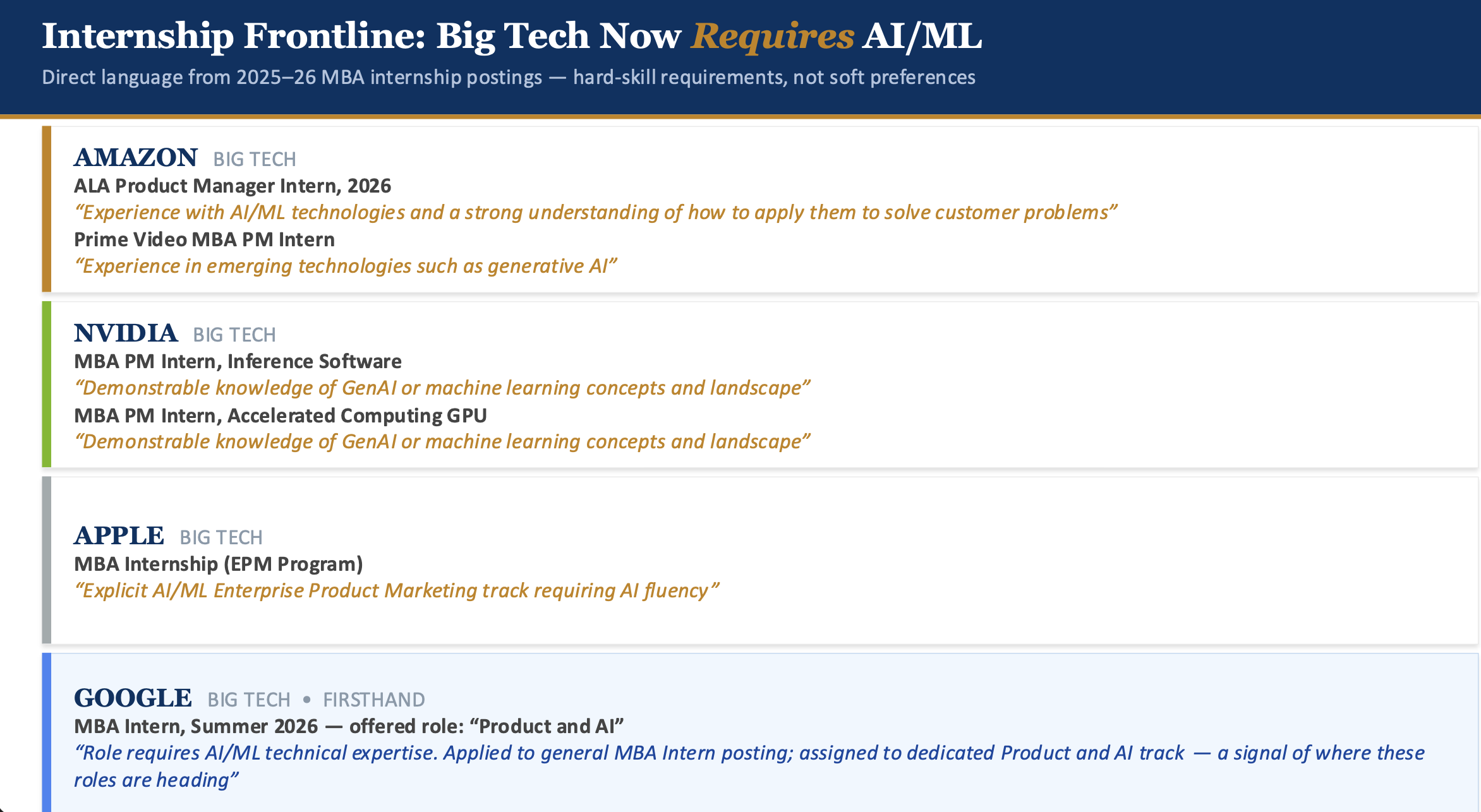
Big Tech Now Requires AI/ML

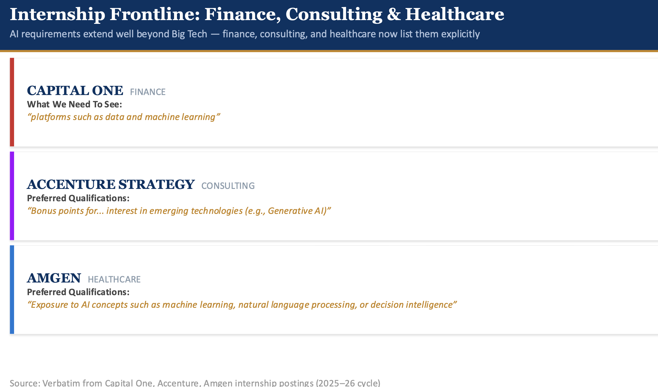
Not Just Tech — Finance, Consulting, Healthcare Too

What Today’s Class Gives You

What it takes to build an in-house model — what data you need, how it’s collected and labeled, how training actually works, and what’s realistic vs a money pit. This class covers the full pipeline so you can evaluate build vs buy with real understanding
Why data quality matters more than quantity — not just “do we have data?” but how it’s labeled, who labeled it, what biases it carries, and why dumping more data into a model doesn’t automatically make it better
How models learn — training, loss, overfitting — so when an engineer says “the model is overfitting” or “we need cleaner labels,” you understand the actual problem and can make a call
What neural networks, attention, and transformers are — the engine behind every AI product you’ll work with, and why architecture choices affect cost, speed, and accuracy
The vocabulary — embeddings, parameters, fine-tuning, tokens, inference — so you can speak with engineers directly and ask the right questions

Important

I’m not teaching you to be ML engineers. I’m going over the concepts so you understand them well enough to make real decisions — knowing the limitations of AI instead of assuming you understand it from one article or a case study.

Why AI Instead of Code?

Why Can’t We Just Code All the Rules?

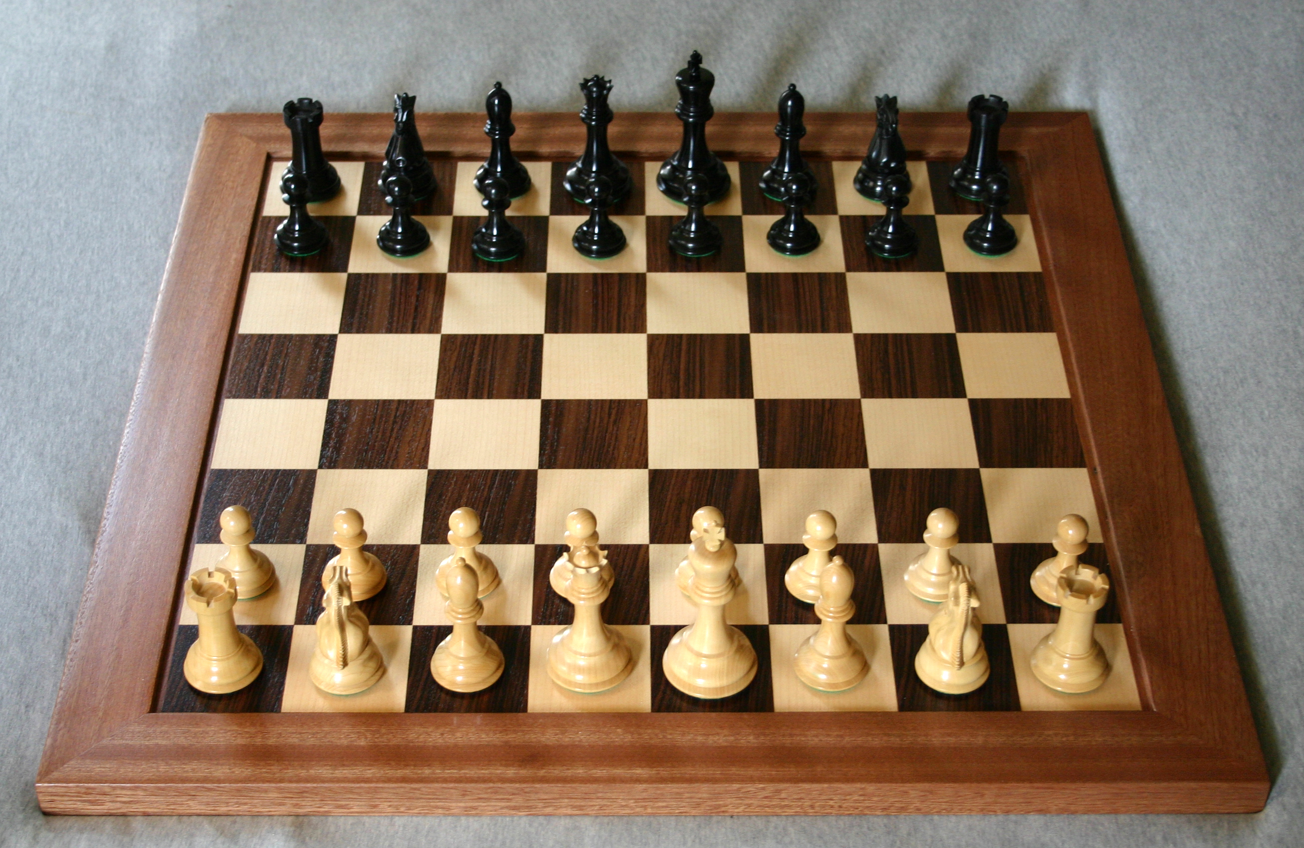
Chess has simple rules. A finite board. A finite set of pieces. Couldn’t we just program every possible move?

	Number	Scale
Possible chess games	10¹²⁰	a 1 followed by 120 zeros

Atoms in the universe

10⁸⁰

a 1 followed by 80 zeros

Chess has a trillion trillion trillion times more possible games than there are atoms in the universe.

You cannot brute-force chess. This is why we need AI.

AI Feels Like an Alien Oracle…

It’s not magic. It’s statistics, linear algebra, and calculus — the same math from Data & Decisions — running at a scale no human could do by hand. By the end of today, you’ll understand exactly how it works.

Condensation of Knowledge

A chess grandmaster doesn’t memorize every possible game. They develop intuition — compressed patterns from thousands of games.

AI does the same thing, but as math.

Take massive amounts of data (millions of games, images, documents)
Condense the patterns into a mathematical model
The model is a compressed representation of everything it learned
It can then make predictions on situations it’s never seen before

Tip

This is the core idea of AI: learn patterns from data and compress them into math, instead of hand-coding every rule.

AI Is Older Than You Think

AI: A 70-Year Journey

AI Was Born in the 1950s

AI was coined in 1956 — before personal computers, before the internet. It’s a 70-year-old math problem that finally got enough compute to work.

Year	Milestone	Why It Matters
1956	AI coined at Dartmouth	Researchers thought human-level AI was 20 years away
1960s–80s	AI Winters	Hype → disappointment → funding dried up. Twice.
1997	Deep Blue beats Kasparov	Brute force — evaluated 200M positions/sec. Not “learning.”
2012	Deep Learning revolution	AlexNet + GPUs proved neural networks work at scale
2017	Transformers & Attention	“Attention Is All You Need” — the architecture behind every modern AI
2022	ChatGPT	100M users in 2 months. AI went from research to daily tool.

What’s different now? Scale. We finally have enough data, enough compute, and the right architecture. The ideas aren’t new — the resources are.

The AI Landscape — What’s Inside What

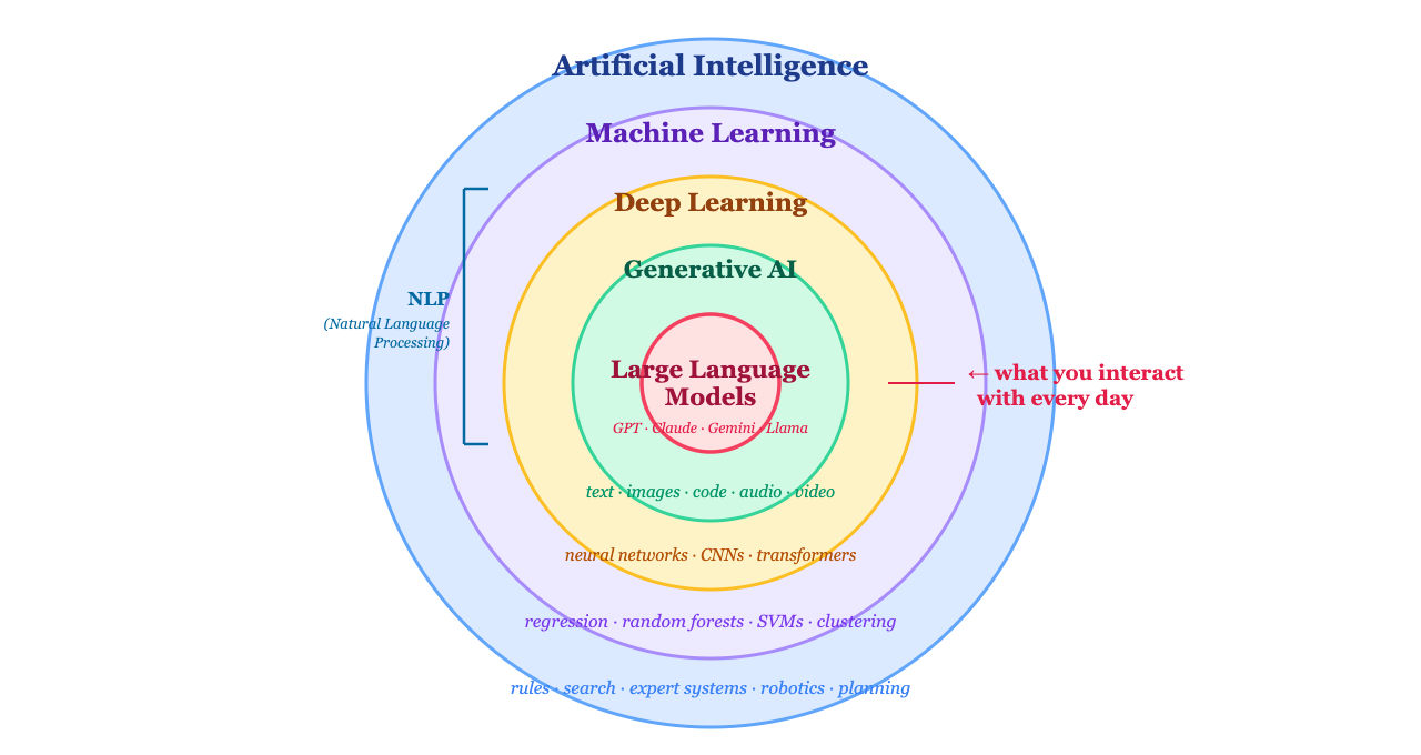
AI is the broadest field — any technique for machines to perform tasks that normally require human intelligence
Machine Learning is the subset that learns from data instead of being explicitly programmed
Deep Learning uses neural networks with many layers — the engine behind modern AI
Generative AI creates new content — LLMs are the subset specialized in language
When people say “AI” today, they usually mean the innermost layer — but the field is much larger

It’s Math, Not Computer Science

AI’s roots are in statistics, probability, linear algebra, and optimization — not programming.

If you have a background in econ, stats, or finance — you’re actually better equipped than most CS grads to understand the core ideas.

Remember Data and Decisions? You already know more AI than you think:

You Already Know	In AI, That’s
Gaussian distributions	How models represent uncertainty and noise
Linear regression	A machine learning algorithm (literally)
Optimization / minimizing loss	Exactly how neural networks learn

AI is applied math at scale. You’ve been doing the fundamentals already.

The Three Forms of Learning

Almost all of AI falls into three paradigms:

Form	How It Learns	Example
Supervised	From labeled examples (input → correct answer)	“This email is spam”, “This house sold for $450K”
Unsupervised	Finds patterns in unlabeled data on its own	Customer segmentation, topic discovery
Reinforcement	By trial and error — actions → rewards	Game-playing AI, robotics, ChatGPT’s RLHF

Note

Most of what we’ll cover is supervised learning — it’s the most common and the foundation for understanding the rest. We’ll touch on reinforcement learning (Bellman equation) and unsupervised learning (clustering) later.

The Two Types of Prediction

Classification vs Regression

Almost every ML problem is one of these two:

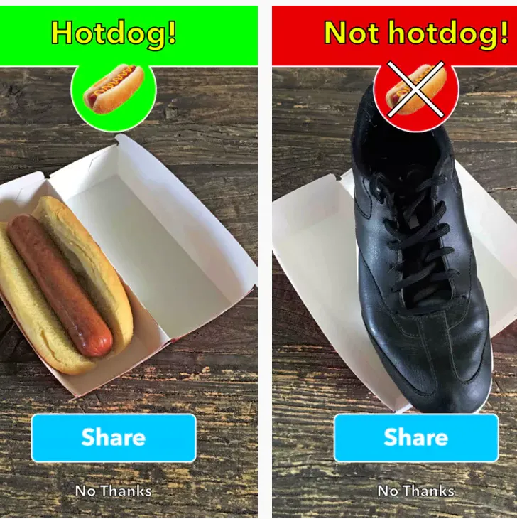
Classification — which category?

Is this email spam or not spam?
Is this image a cat or a dog?
Should we approve or deny this loan?
Will this customer churn or stay?

Regression — what number?

What will this house sell for?
What will the stock price be tomorrow?
How many units will we sell next quarter?
What’s the probability of default?

ML Algorithms — The Quick Tour

Algorithm	Type	How It Works	Good For
Linear Regression	Regression	Fit a line through data	Price prediction, trends
Logistic Regression	Classification	Fit a curve to predict probability	Spam detection, yes/no decisions
Decision Trees	Both	Ask yes/no questions in a flowchart	Interpretable decisions
Random Forests	Both	Many trees vote together	Most tabular data problems
Neural Networks	Both	Layers of connected neurons	Images, text, complex patterns
SVMs	Classification	Find the best boundary between groups	Small datasets, high dimensions

Note

You don’t need to memorize these. The point: there’s a toolbox of algorithms, each suited to different problems. Modern AI is mostly neural networks, but the simpler ones still matter.

Training a Model

Labeled Data

To train a model, you need examples with known answers.

1,000 photos each labeled “cat” or “dog”
10,000 emails each labeled “spam” or “not spam”
50,000 house sales with the actual price

This is called supervised learning — the model learns from examples where we already know the right answer.

Important

Labeling is expensive. Someone has to look at each photo and say “that’s a cat.” This is often the biggest bottleneck in ML — not the algorithm, but getting enough labeled data.

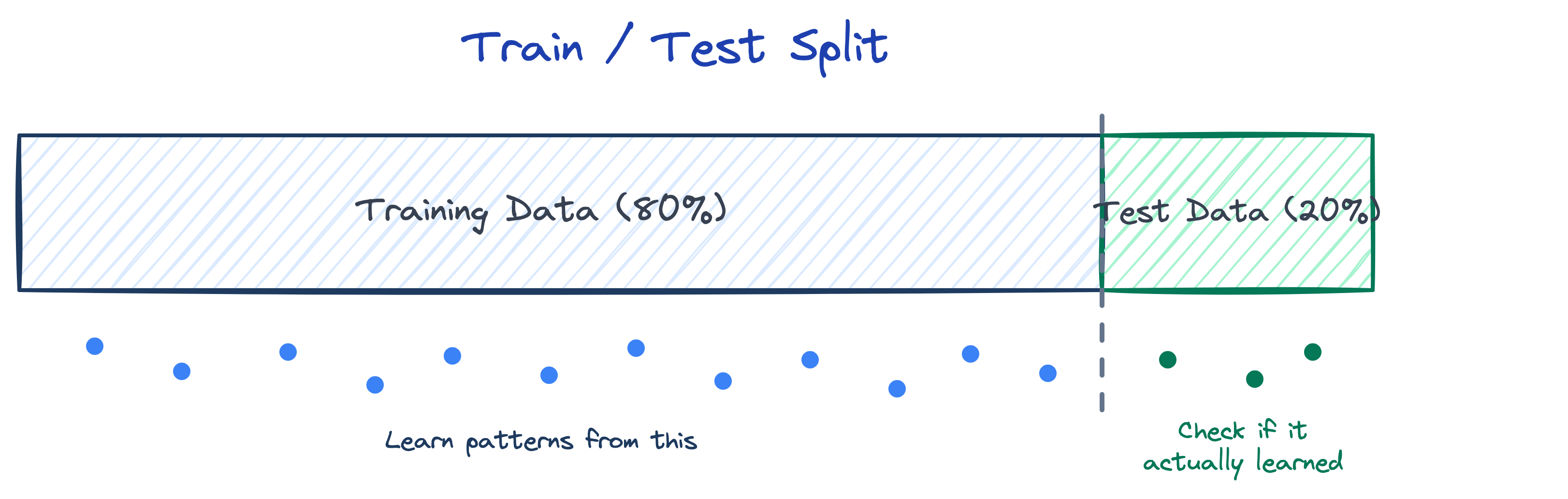
Train / Test Split

You never test a model on the same data it learned from.

Split your data:

~80% Training set — the model learns patterns from this
~20% Test set — check if it actually learned (held back, never seen during training)

Warning

Testing on training data is like grading a student with the exact answer key they studied from. Of course they’ll score 100% — but they haven’t actually learned anything.

What Is Loss?

Every model has settings it adjusts during training. But how does it know if those settings are any good? It needs to measure how wrong it is.

That’s what a loss function does.

Example: you predict a house sells for $300K. It actually sold for $450K. Your error is $150K.

A loss function turns that error into a single number. The most common one:

\[\text{Squared Error} = (\text{predicted} - \text{actual})^2\]

Why squared? A $150K miss is much worse than three $50K misses. Squaring penalizes big mistakes more.

Note

This is exactly what you did in Data and Decisions — minimizing the sum of squared errors in linear regression. Every ML algorithm does the same thing: make predictions, measure loss, try to reduce it.

Loss in Action — Starting With a Guess

The model starts with a random line. It’s terrible.

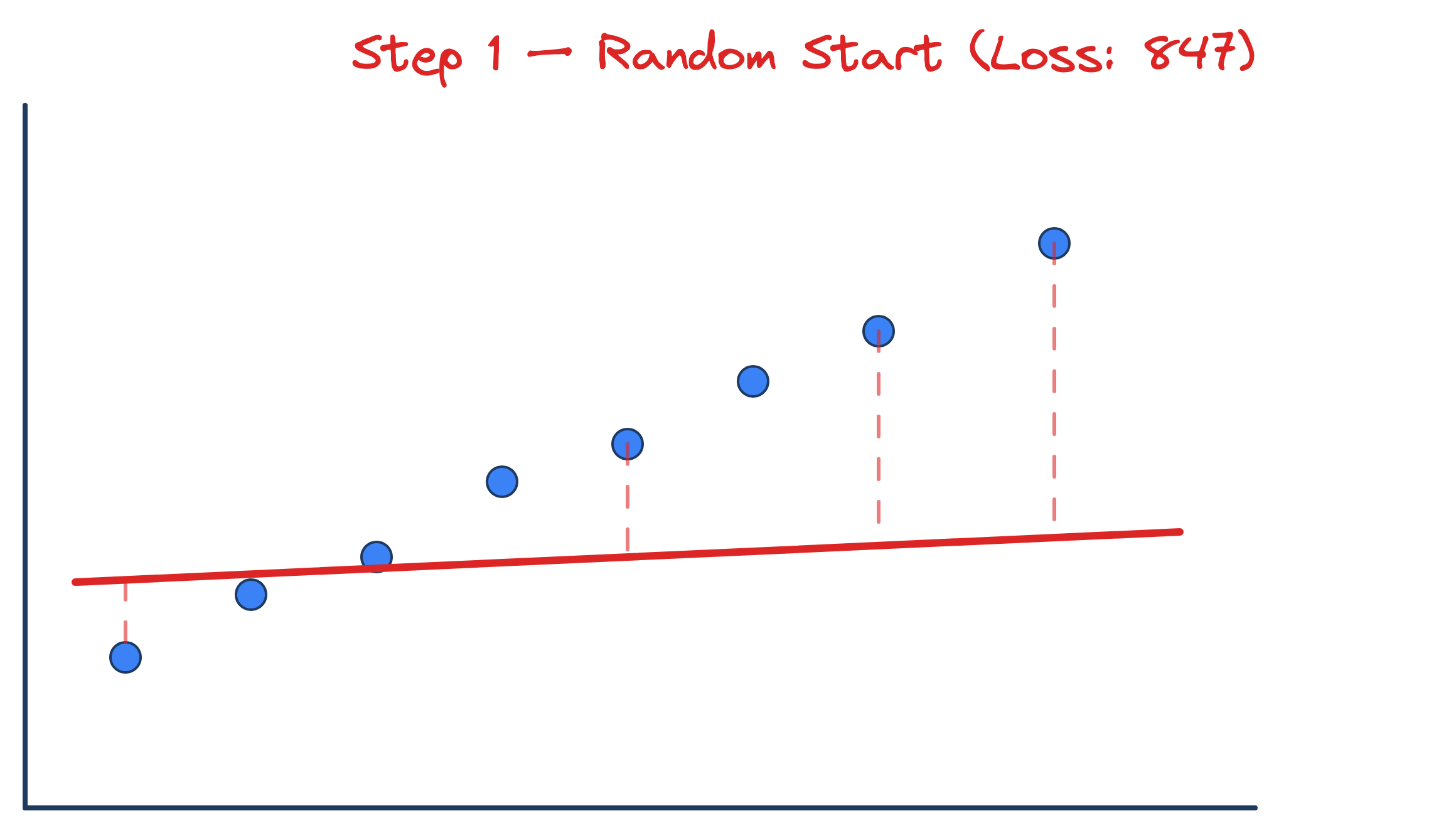
The dashed lines are the errors — the gap between each prediction and the real value. Loss = 847.

How Does the Model Know Which Way to Adjust?

Most points are above the line → the line is too low → tilt it up
Points on the right are much further than points on the left → the slope is too shallow → steepen it
Bigger errors contribute more to the loss (because we square them) → fix the biggest misses first

The errors don’t just tell you “you’re wrong” — they tell you which direction and by how much.

Adjusting — Step by Step

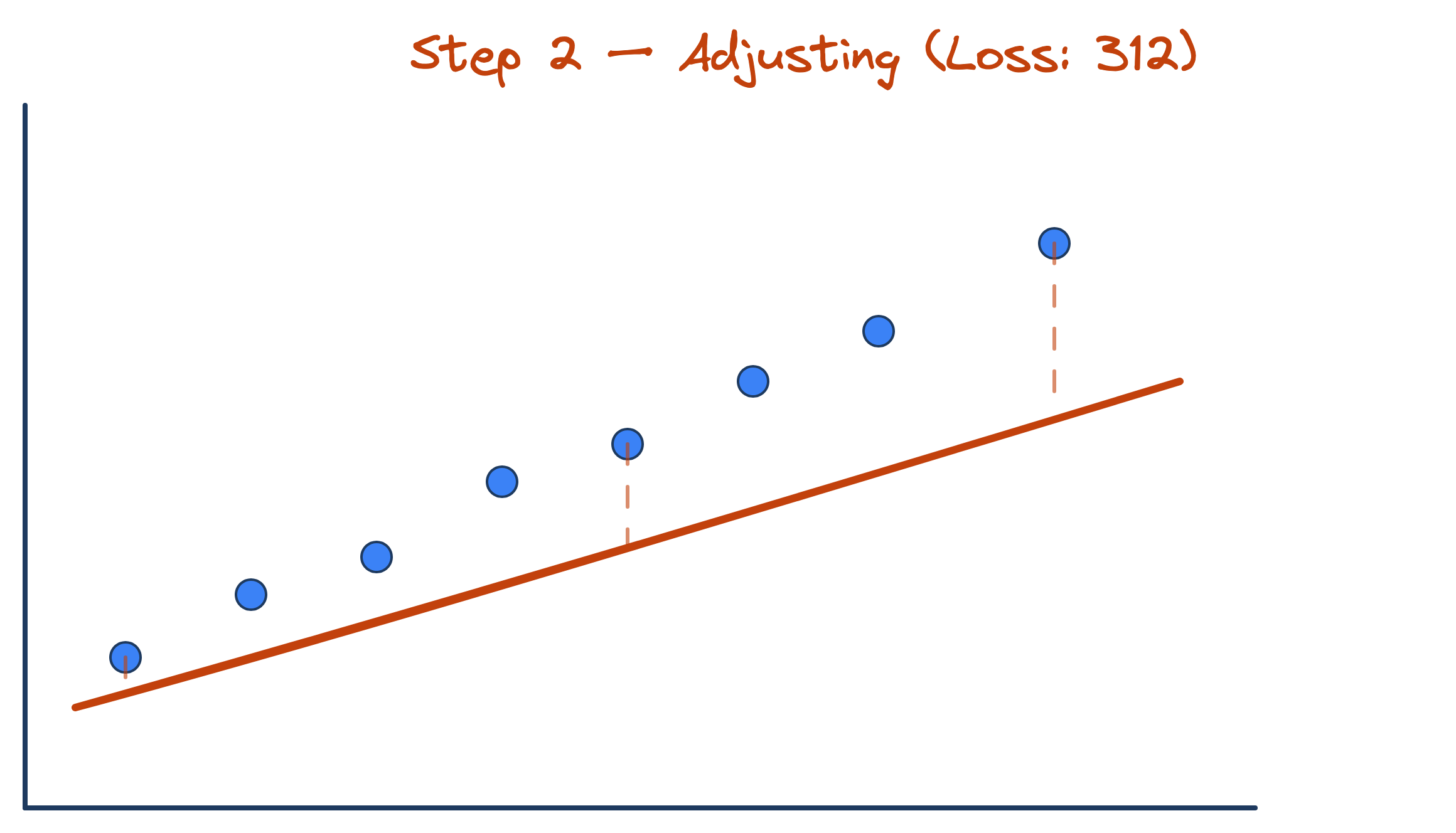
The model tilted the line up and steepened it. Loss dropped from 847 → 312. Better, but still off.

Getting Close

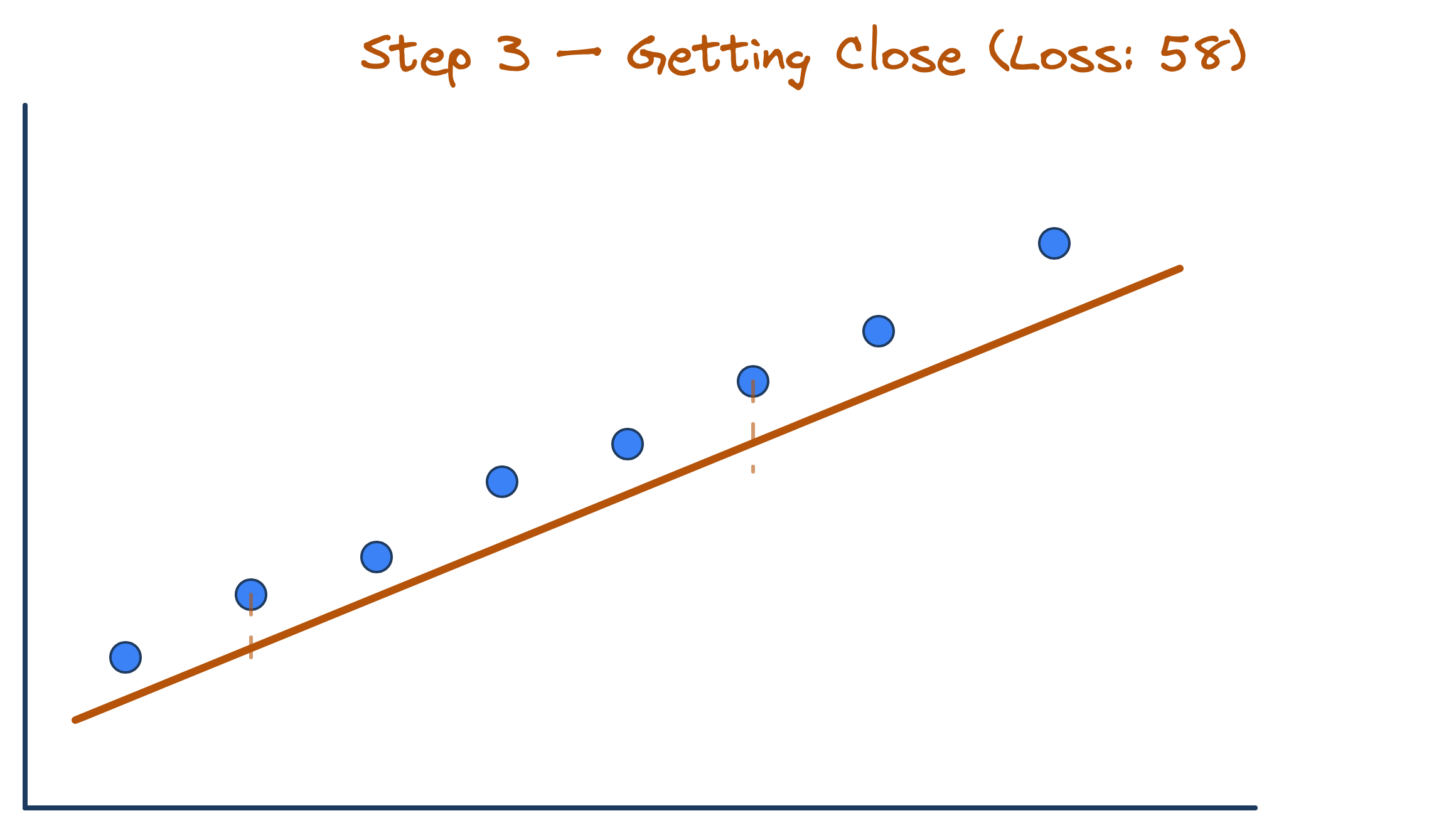
Another adjustment. Loss: 312 → 58. The error lines are barely visible now.

Converged!

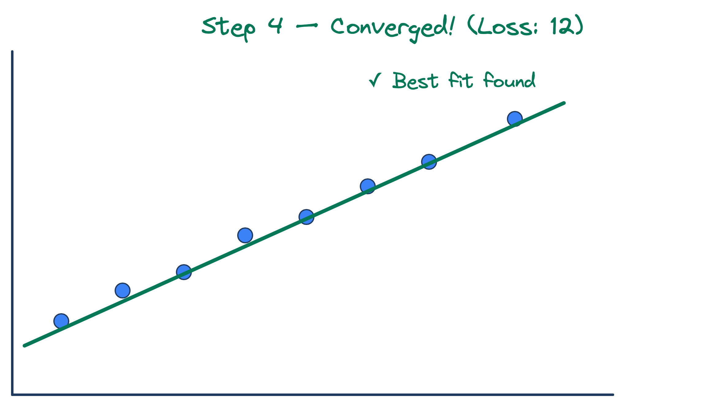
Loss: 12. The line fits the data. This is what “training” looks like — measure error, adjust, repeat.

This Process Has a Name

That cycle — measure the error, figure out which direction to move, take a step, repeat — is called gradient descent.

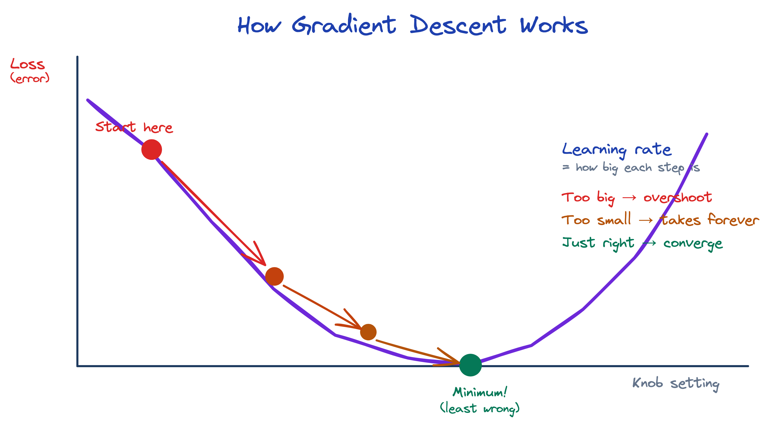
The model starts with random parameters (high on the hill), measures the loss, and takes a step downhill. Repeat until it reaches the minimum.

Local Minima — Good Enough vs Best

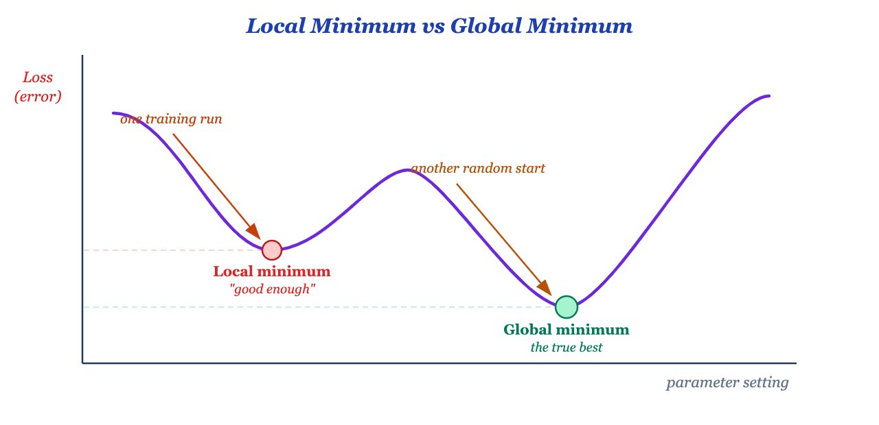
Sometimes gradient descent lands in a valley that looks good enough
But that valley may be only a local minimum, not the true best
That is why we do many training runs with random starts and different scenarios
More attempts increase the chance of finding the real optimum

Overfitting — Memorizing vs Learning

A model that memorizes training data but fails on new data has overfit.

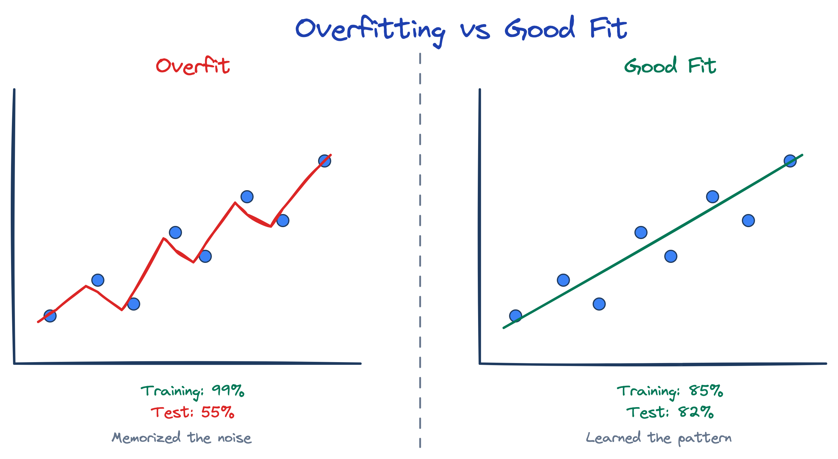
Red line: learned the noise, not the signal
Training: 99%. Test: 55%.

Green line: learned the trend
Training: 85%. Test: 82%. Much better on new data.

Extrapolation — The Danger Zone

Even a model that isn’t overfit can fail outside the range of data it’s seen.

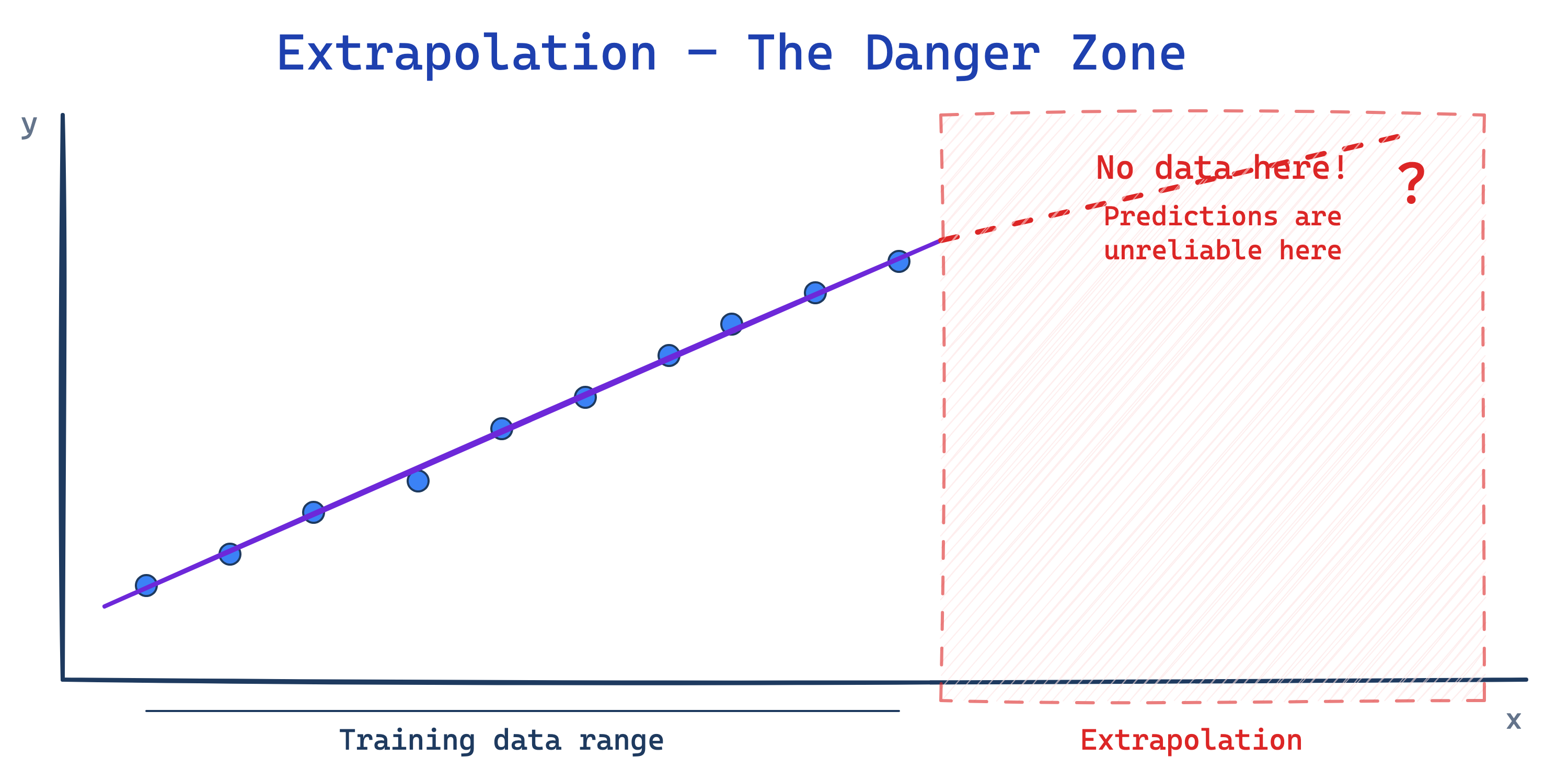
The red zone is not the test set — it’s completely new territory
Houses $200K–$800K → can’t predict $5M mansions

US market data → fails on emerging markets
Models don’t warn you — they give a confident, wrong answer

Decision Trees & Random Forests

Decision Trees — A Flowchart of Questions

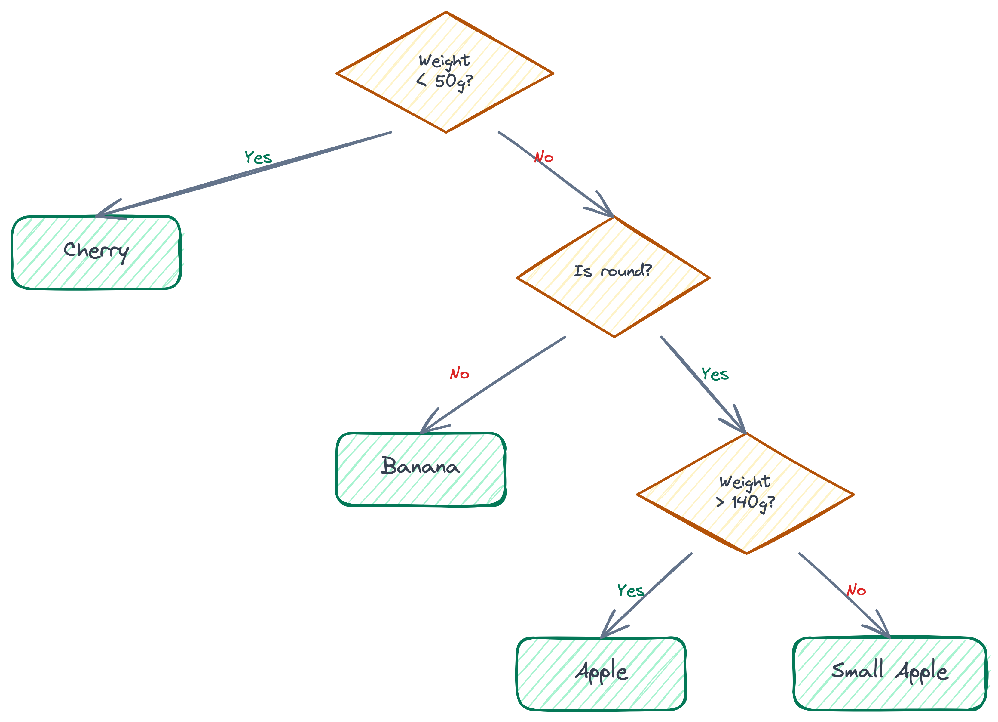
The simplest ML model: ask a series of yes/no questions to classify data.

Is it red? → Apple
Yellow and curved? → Banana
Small and round? → Cherry

Each node asks a question, each branch is an answer, each leaf is a prediction.

How Trees Choose Questions

Think of 20 Questions. You wouldn’t start with “is it a Granny Smith apple?” — that only eliminates one thing. You’d ask “is it a fruit?” — that splits the world in half.

The tree tries every possible question and picks the one that separates the groups most cleanly
A good split: “is it round?” puts all bananas on one side and everything else on the other
A bad split: “is it heavier than 142g?” barely separates anything
The goal: fewest questions to reach the answer — the most efficient path

This “how cleanly does this question split things?” is measured by something called Gini impurity — but the intuition is just: pick the question that eliminates the most possibilities in one step.

Random Forests — Wisdom of the Crowd

One tree is good. But it can overfit.

The solution: build many trees and let them vote.

A Random Forest builds hundreds of decision trees, each trained on a random subset of the data. The final prediction is the majority vote.

Note

Each tree might make mistakes, but they make different mistakes. When you combine their votes, errors cancel out and correct answers reinforce each other. This is called ensemble learning.

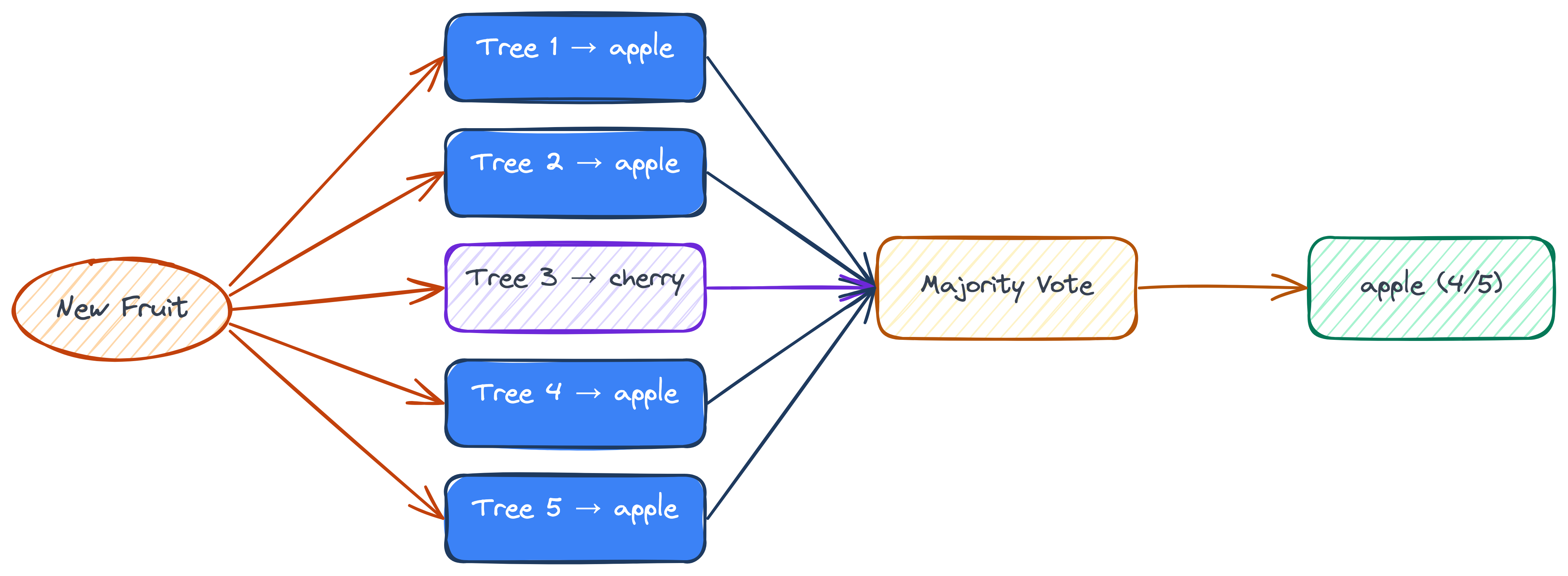
Random Forest: Many Trees Vote

Neural Networks

The Artificial Neuron

Neural networks are inspired by the brain — networks of simple units (neurons) that can learn complex patterns when connected together.

A single neuron does three things:

Takes inputs (numbers)
Multiplies each input by a weight (how important that input is)
Adds a bias, applies an activation function, and produces an output

A Single Neuron in Action

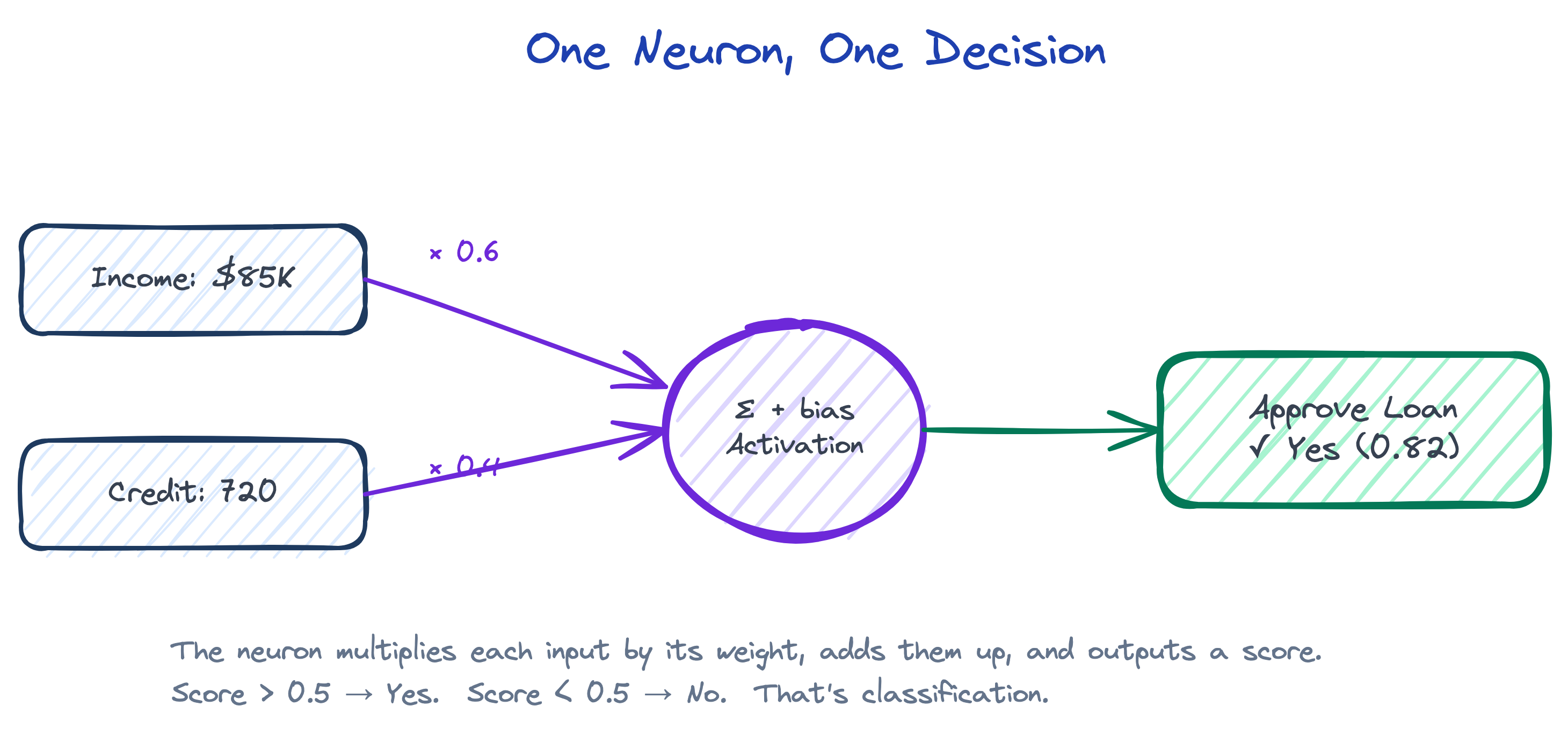
One neuron, one decision: take inputs, multiply by weights, output a score. Score > 0.5 → Yes. Score < 0.5 → No. That’s classification. One neuron isn’t smart — but millions together can recognize faces, translate languages, and write code.

Inspired by the Brain

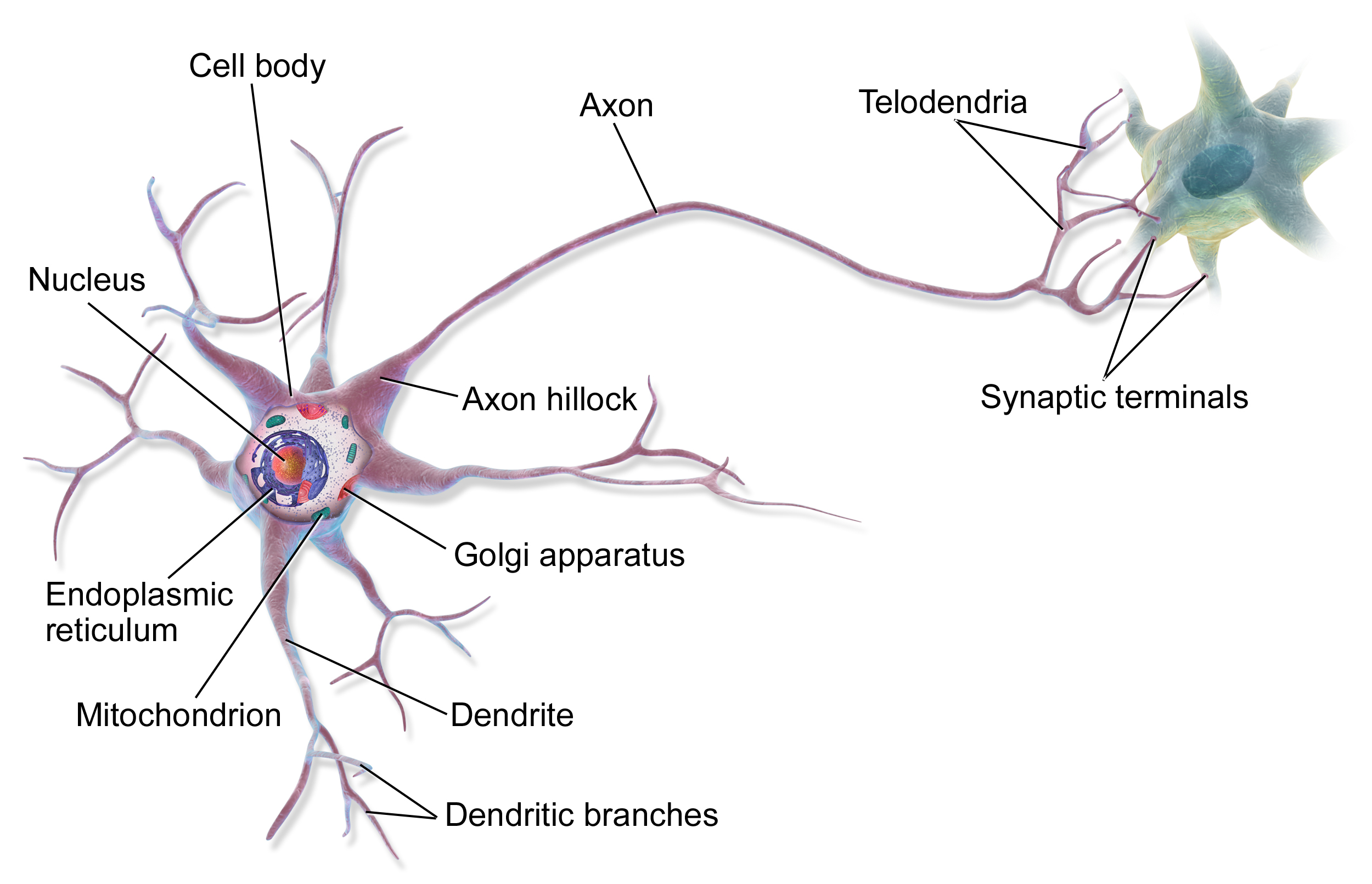
Dendrites receive signals → cell body processes → axon sends output to the next neuron

Inputs × weights → activation function → output to the next layer

This isn’t a coincidence. Neural networks were designed to mimic the brain. Your brain learns by adjusting the strength of connections between neurons — exactly what training does with weights. Both are pattern recognition machines, one biological, one mathematical.

One Neuron → A Network

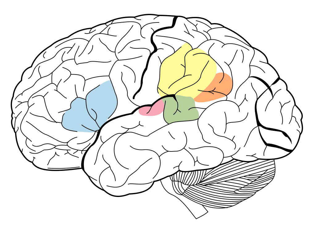
86 billion neurons, each connected to thousands of others. You think, remember, and recognize patterns through these connections.

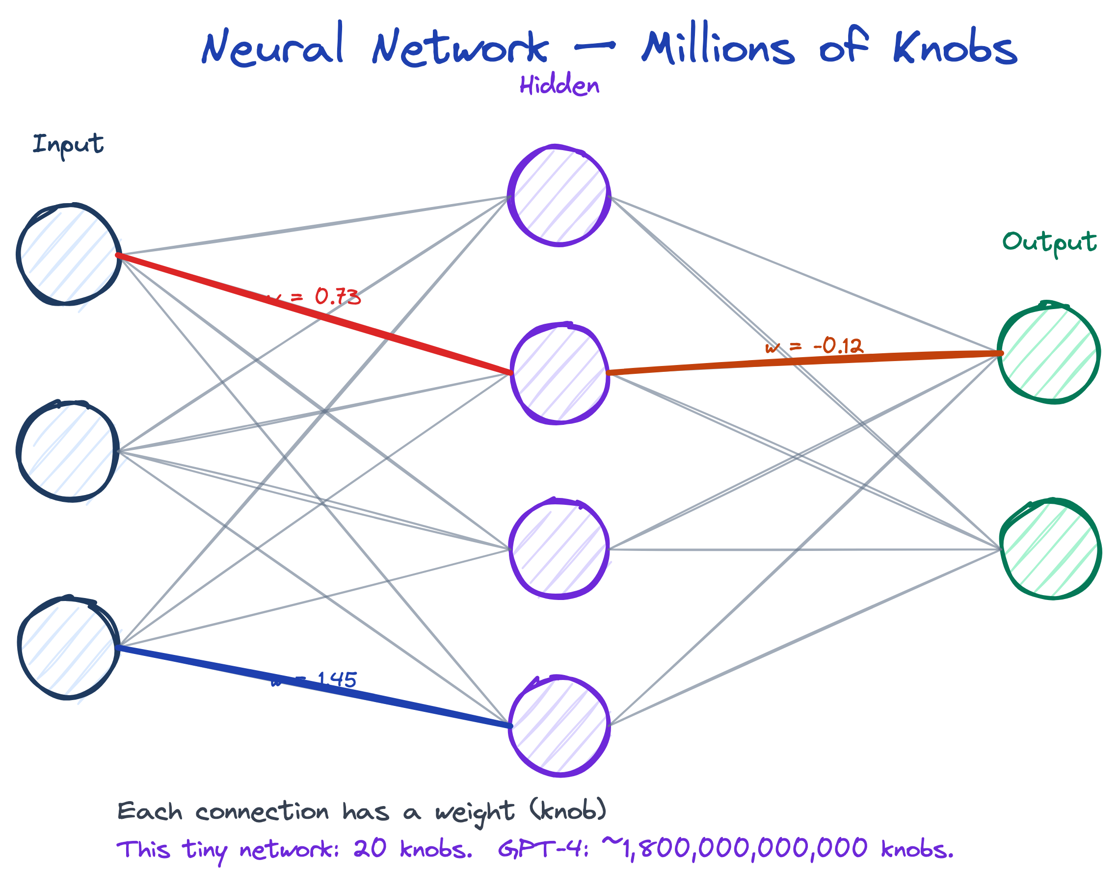
An artificial neural network: layers of nodes, each connected to the next. Every connection has a weight — a number the model adjusts during training.

A single neuron is simple. But billions of them connected together — that’s where intelligence emerges. Same principle, biological or artificial.

How a Neural Network Learns

Think of it like a factory assembly line — a product passes through stations, and when the result is bad, you trace backward to find the fault:

Forward pass — raw materials move through each station in order. Each station does its job. A product comes out at the end.
Calculate loss — quality inspection checks the product. How defective is it? (Same loss from earlier — a single number for “how wrong.”)
Backpropagation — trace backward through the stations: which station contributed most to the defect? Station 3’s temperature was off, station 5’s timing was wrong.
Gradient descent — adjust each station’s settings proportionally to how much it caused the defect. Big cause → big adjustment.
Repeat — run the line again. Inspect. Trace back. Adjust. Thousands of times until the products are good.

The Training Loop

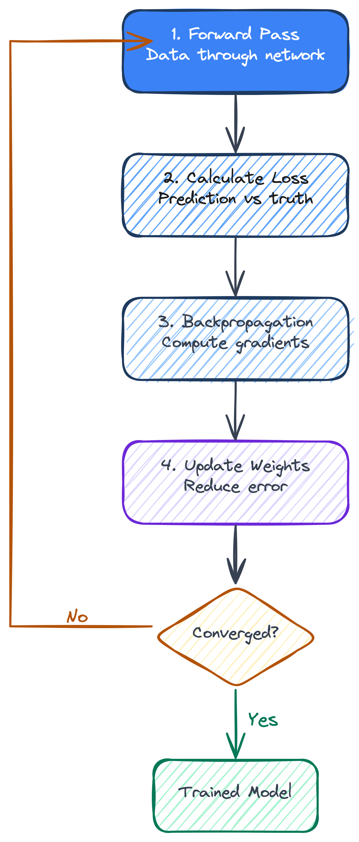
This is the same cycle every ML model uses — predict, measure loss, adjust. Neural networks just do it with millions of weights instead of one line through data.

What’s Actually Being Adjusted?

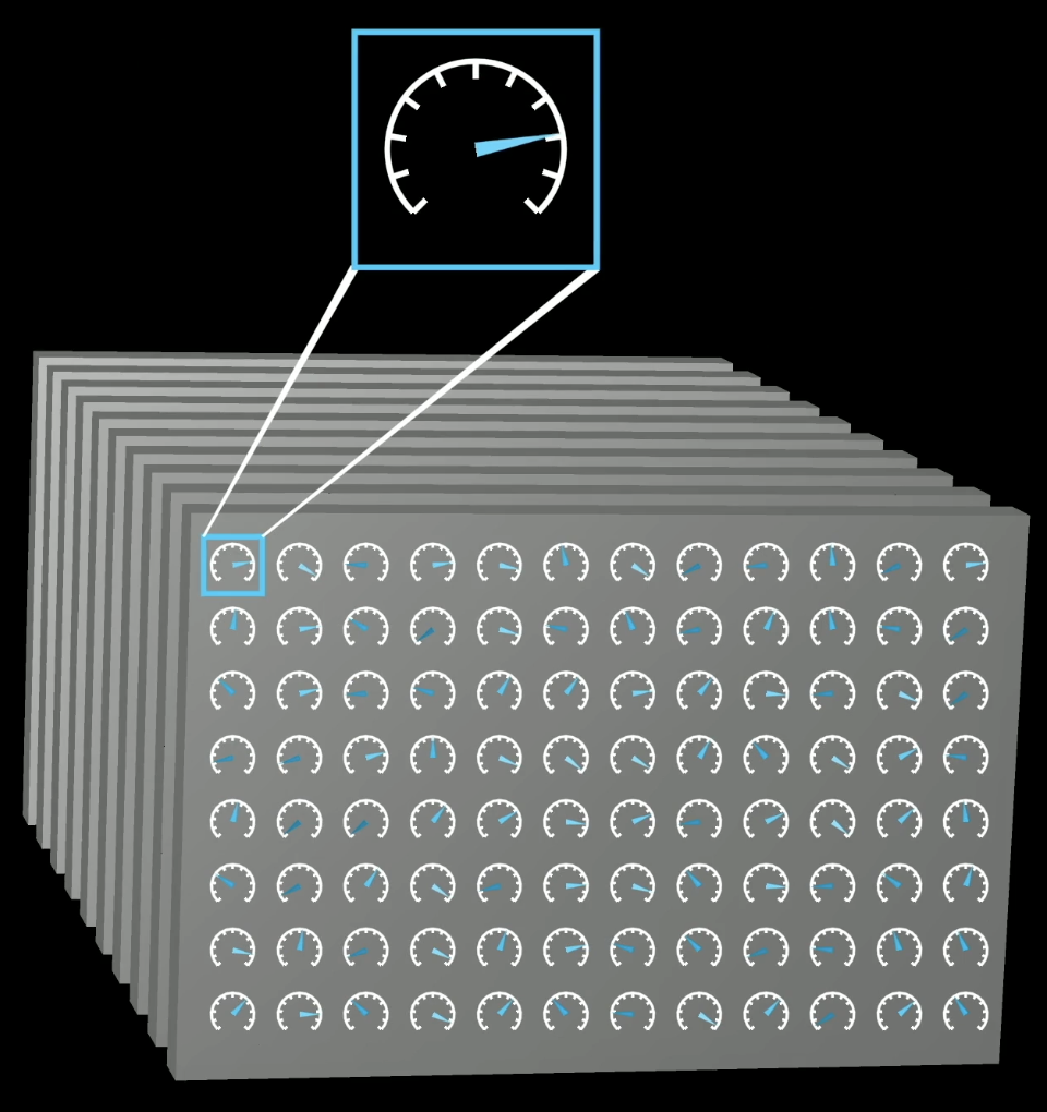
Every line connecting two neurons is a weight — a knob the model adjusts during training. This tiny network has 20 knobs. GPT-5 has an estimated 5 trillion.

Parameters vs Hyperparameters

Not all knobs are the same. There are two kinds:

Parameters (the model learns these)

The weights between neurons
Adjusted automatically by gradient descent
Millions or billions of them
You never set these by hand

Hyperparameters (you choose these)

Learning rate — how big each step is
Number of layers — how deep the network
Number of neurons per layer — how wide
How long to train — number of epochs

Note

Parameters are what the model figures out. Hyperparameters are the decisions you make before training starts. Picking good hyperparameters is part art, part science — and one of the key skills in ML.

Deep Neural Networks

Why Depth Matters

A single neuron can learn simple patterns. But complex patterns need many layers — that’s a deep neural network.

Take a network that recognizes photos of faces. You feed it raw pixels. It has never been told what a “face” is. But each layer learns something more complex than the last:

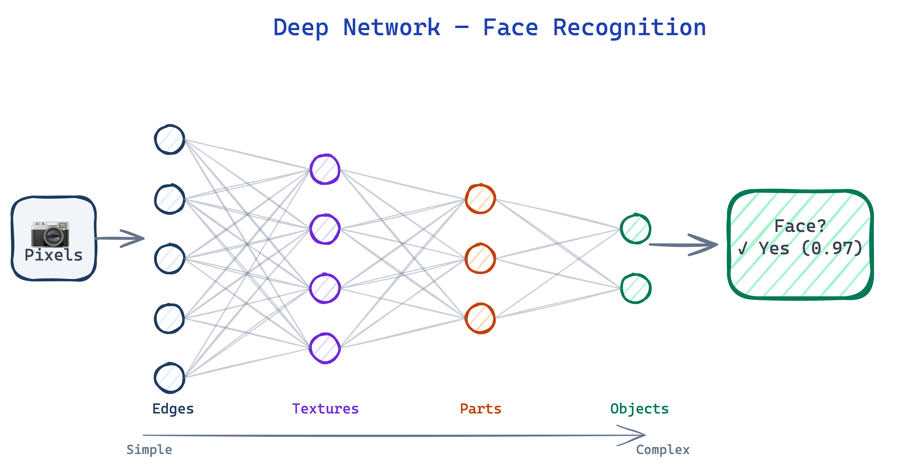
Layer 1: Spots edges — light vs dark boundaries in the pixels
Layer 2: Combines edges into textures — skin, hair, fabric
Layer 3: Groups textures into parts — “this looks like an eye”, “that’s a nose”
Layer 4: Assembles parts into a face — “this is a person”

Nobody programmed “look for eyes.” The network figured it out from millions of photos. More layers = more abstraction. This only became practical when GPUs gave us the power to train these in parallel.

Reinforcement Learning

Learning by Trial and Error

Decision trees and neural networks learn from labeled data (supervised learning). But what if there’s no labeled data? What if an agent has to learn by doing?

That’s Reinforcement Learning (RL).

In supervised learning, loss tells you how wrong you are. In RL, reward tells you how right you are — same coin, different side.

Tip

RL is like training a dog. The dog (agent) tries something (action), and you give it a treat (positive reward) or say “no” (negative reward). Over time, the dog learns which behaviors earn treats.

States, Actions, Rewards

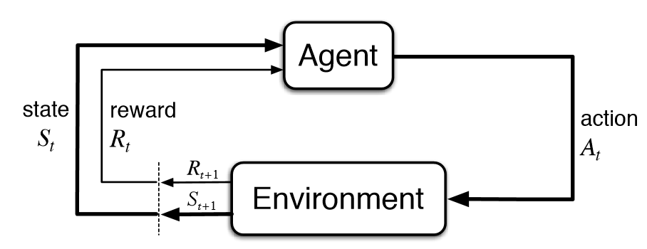
Action (A_t) = what the agent chooses to do (accelerate, brake, turn left)
Reward (R_t) = feedback on how good that action was (+1 smooth driving, -100 collision)
State (S_t) = a snapshot of the world (the environment) right now (speed, position, traffic light, pedestrians)
t = the time step. At t=1 the car is at a red light (S₁), it brakes (A₁), gets +1 (R₁). Light turns green → new state S₂, new action A₂, new reward R₂. The loop continues.

The Bellman Equation

This one equation underlies most of AI:

\[\Huge V(s) = \max_a \left[ R(s, a) + \gamma \cdot V(s') \right]\]

In plain English:

“The value of where I am = the best reward I can get now + how good the place I’ll end up is.”

From chess engines to self-driving cars to ChatGPT’s RLHF training — this is the foundation.

The Grid World Challenge

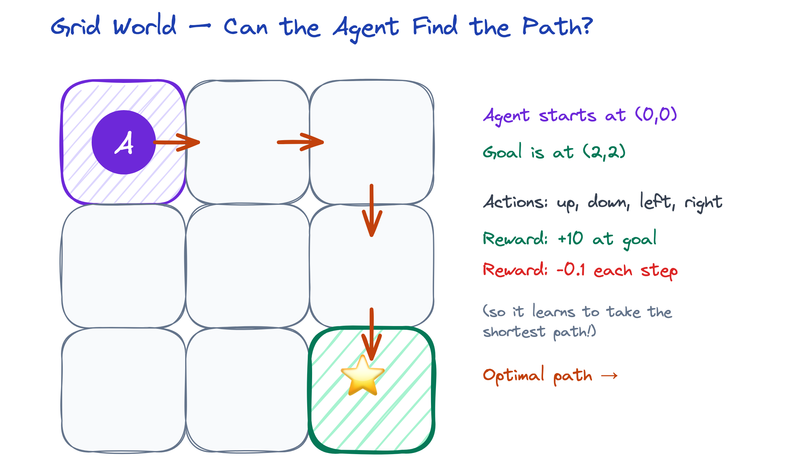
The agent starts at (0,0) with no knowledge of the grid. It doesn’t know where the goal is. It just tries actions, gets rewards, and learns. Can it find the shortest path on its own?

See It Work: Grid World

Let’s run it — the agent learns entirely by trial and error:

Note

Nobody told the agent the rules. It figured out the shortest path by exploring, failing, and learning from rewards. This same principle trained AlphaGo to beat the world Go champion.

Unsupervised Learning

Finding Patterns Without Labels

What if you don’t have labeled data? Unsupervised learning finds structure on its own.

Clustering: group similar things together — customer segments, topic discovery, anomaly detection
Dimensionality reduction: compress 1,000 features into 10 that capture the same information
Recommendation systems: “users like you also liked…” — no one labeled the recommendations

Note

Unsupervised learning is how Netflix recommends shows, how banks detect fraud, and how Google organizes search results. It’s everywhere — and it doesn’t need a single label.

Teaching Machines to Read

Why Language?

So far, every model we’ve seen works with numbers — house prices, pixel values, grid positions.

But the biggest AI breakthroughs came from teaching machines to read text
Why? The internet is mostly text. Trillions of words, freely available
If you can teach a machine to read, you can train it on the entire internet

Note

This is exactly what happened. The shift from images to language is what gave us ChatGPT, Claude, and every modern AI assistant.

The Problem: Words Aren’t Numbers

How do you feed words into a neural network that only understands numbers?

You convert words into vectors — lists of numbers that capture meaning.

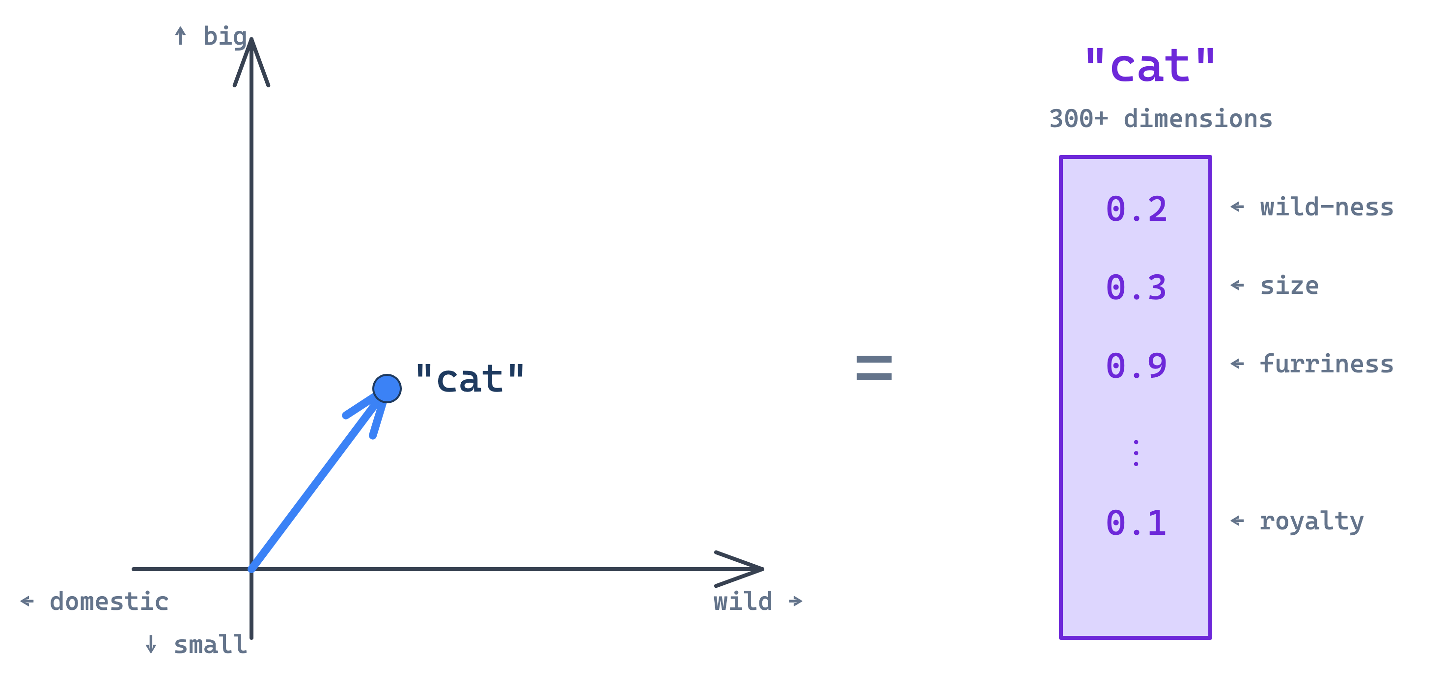
Warning

This is simplified! Real dimensions aren’t neatly labeled “furriness” or “size.” The model discovers its own abstract axes through optimization — each one blends many concepts. But the intuition holds: similar words end up as nearby points.

Words as Points in Space

Word2Vec (2013) learned that words in similar contexts get similar vectors.

“The ___ sat on the mat” → cat, dog, child all fit → similar vectors.

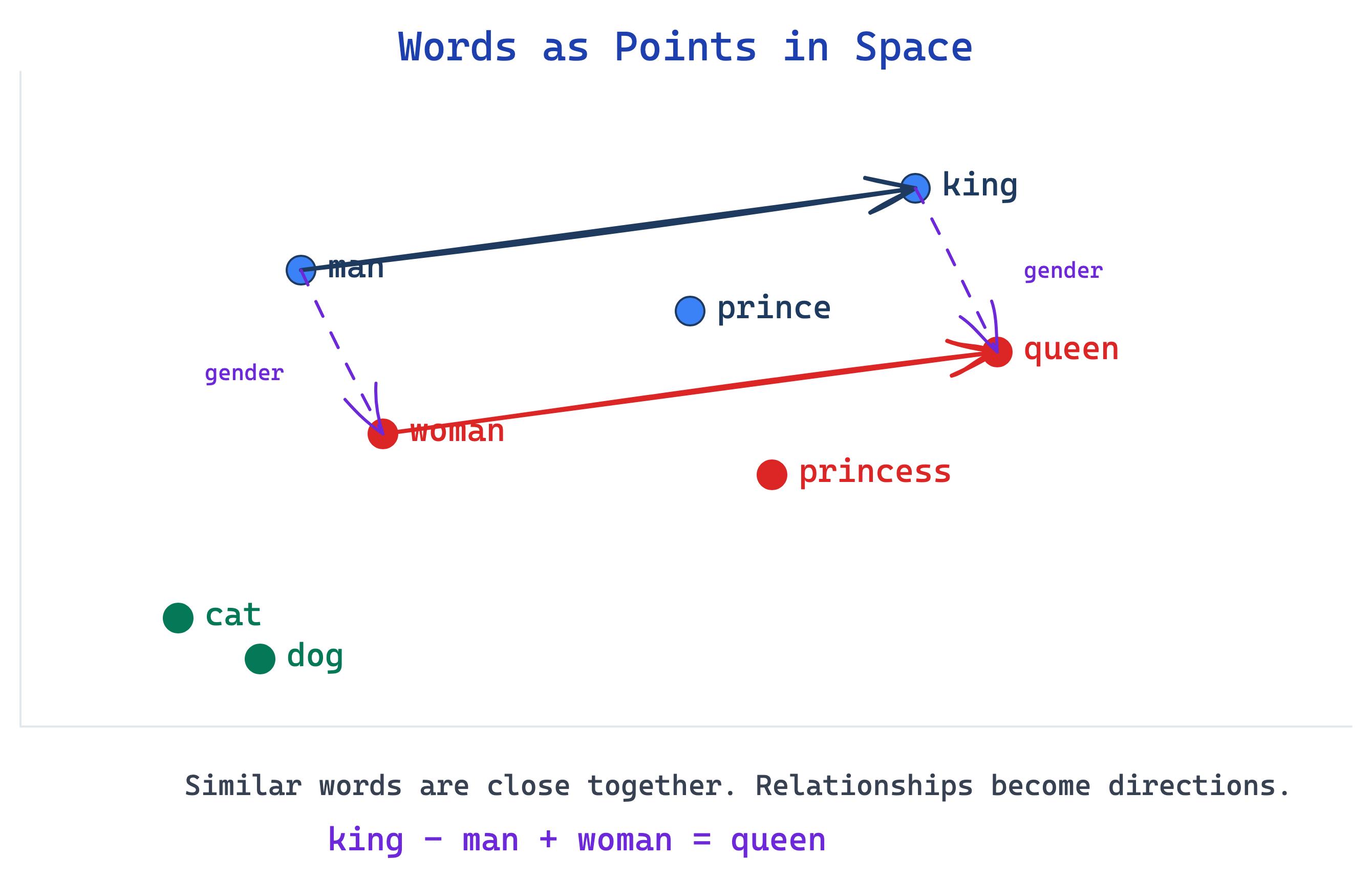
Words with similar meanings cluster together. Relationships like gender, royalty, and age become directions you can navigate with math.

Important

king - man + woman ≈ queen

The model learned gender as a direction in vector space, without anyone teaching it!

Explore Word Embeddings in 3D

Tip

Click Word2Vec 10K on the left. Search for “king” — then look at what’s nearby. Try toggling between PCA and t-SNE projections.

From Words to Tokens

Modern LLMs don’t use word-level embeddings. They use subword tokenization (BPE):

“unbelievable” → [“un”, “believ”, “able”]
“ChatGPT” → [“Chat”, “G”, “PT”]

This handles rare and new words gracefully — even words the model has never seen can be broken into familiar pieces.

Note

Embeddings are the bridge between human language and neural networks. The discovery that word relationships are captured as directions in vector space was one of the key insights that led to modern NLP and LLMs.

Sequences & Attention

The Problem with Order

Regular neural networks treat each input independently. But what about data where order matters?

“Dog bites man” vs “man bites dog” — same words, opposite meaning
“I didn’t say he stole the money” — stressing different words changes the meaning entirely
A stock price today depends on yesterday’s price, which depends on the day before
The word “bank” means something different after “river” vs after “investment”

Neural networks that look at inputs one at a time, independently, can’t understand any of this. They need memory.

RNNs — Adding Memory

Recurrent Neural Networks (RNNs) process sequences one step at a time, passing a “memory” forward to the next step.

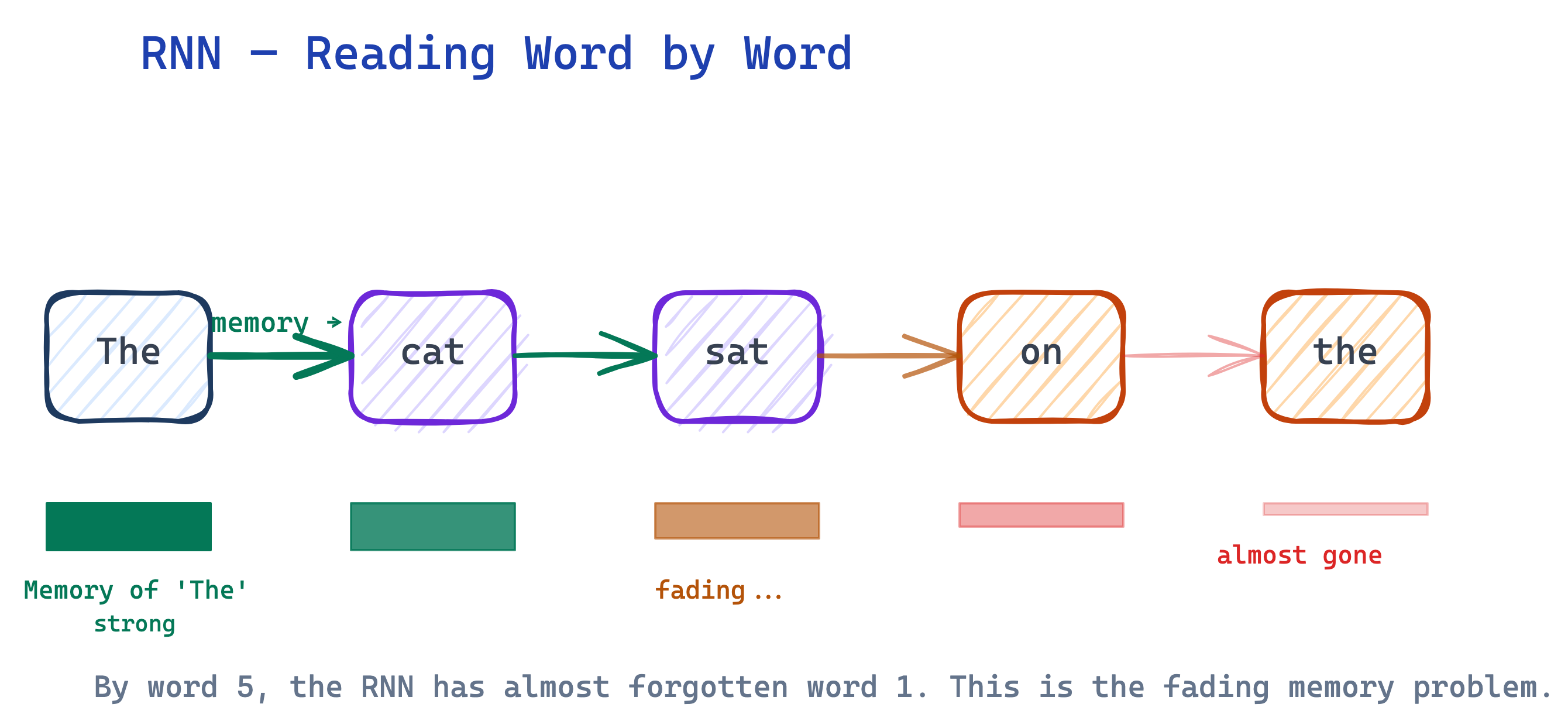
The memory arrows get thinner — by word 5, the RNN has nearly forgotten word 1. And each step waits for the previous one, so it’s slow.

“Attention Is All You Need” (2017)

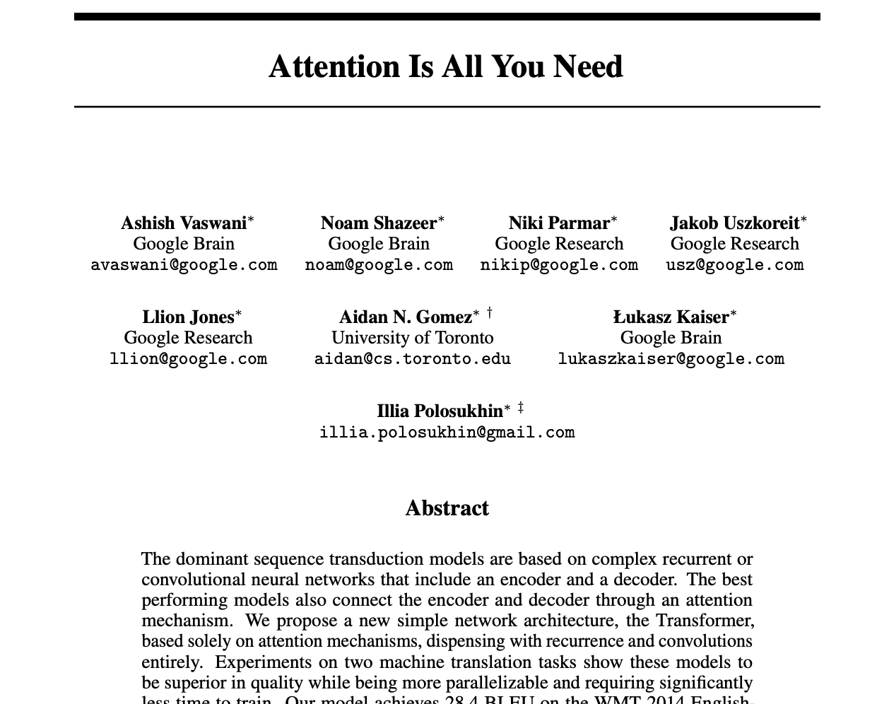
In 2017, Google researchers published arguably the most important AI paper of the decade. The solution to RNNs forgetting and being slow? Don’t process words one at a time at all.

They introduced the Transformer — built entirely on a mechanism called attention, with no recurrence. Every major AI model today — GPT, Claude, Gemini, LLaMA — is a transformer.

Attention: Every Word Looks at Every Other Word

What if, instead of passing a fading memory forward, the model could look at every word at once and decide which ones matter?

That’s attention — each word asks: “who in this sentence is relevant to me?”

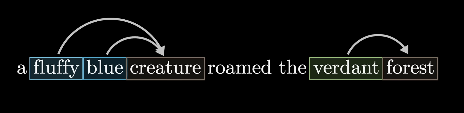
“creature” attends to “fluffy” and “blue” — they describe it. “forest” attends to “verdant.” Each word pulls in context from the words that matter most to it.

Why This Matters: Same Word, Different Meaning

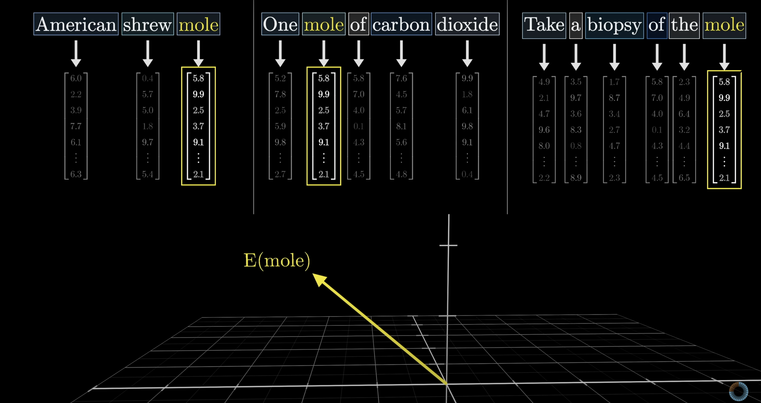
The word “mole” means completely different things depending on context:

“American shrew mole” → a small animal
“One mole of carbon dioxide” → a chemistry unit (6.02 × 10²³)
“Take a biopsy of the mole” → a skin lesion

The embedding for “mole” starts the same in all three sentences. Attention figures out which meaning by looking at surrounding words.

Attention Updates Meaning

After attention, the embedding for “mole” has been pulled toward the right meaning by its context:

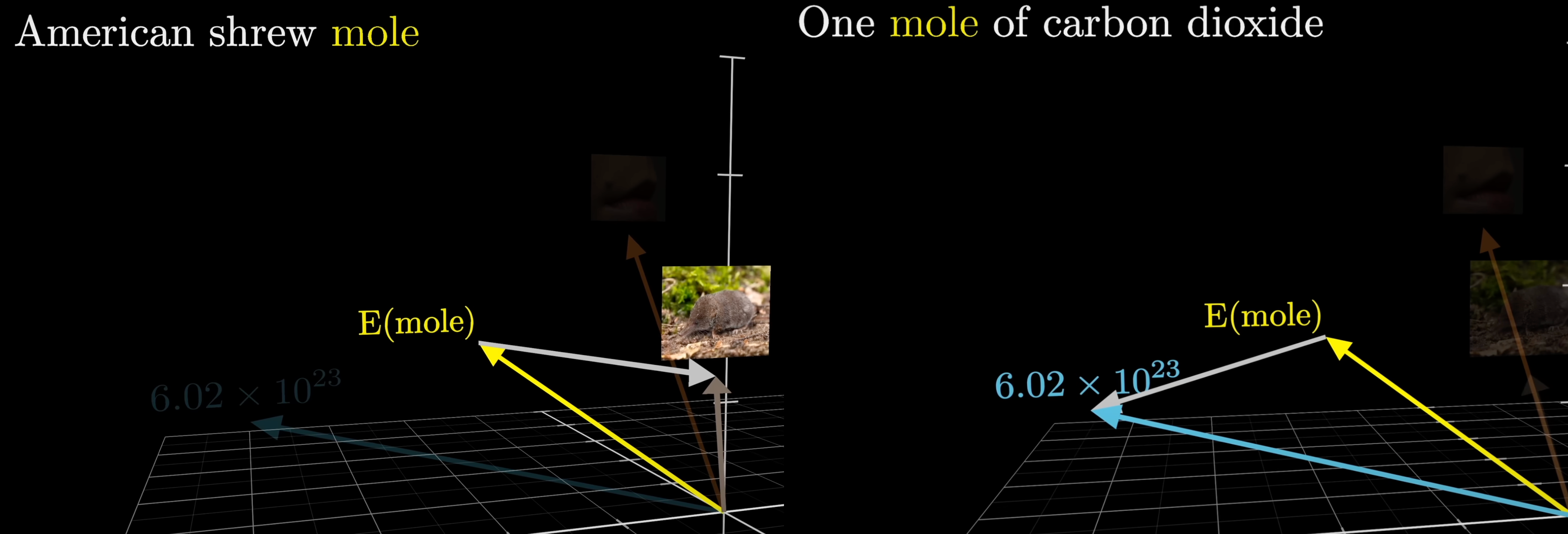
“American shrew” pulls “mole” toward the animal direction. “Carbon dioxide” pulls it toward the chemistry direction. Same starting point, different ending — that’s what attention does.

Transformers

How a Transformer Processes Text

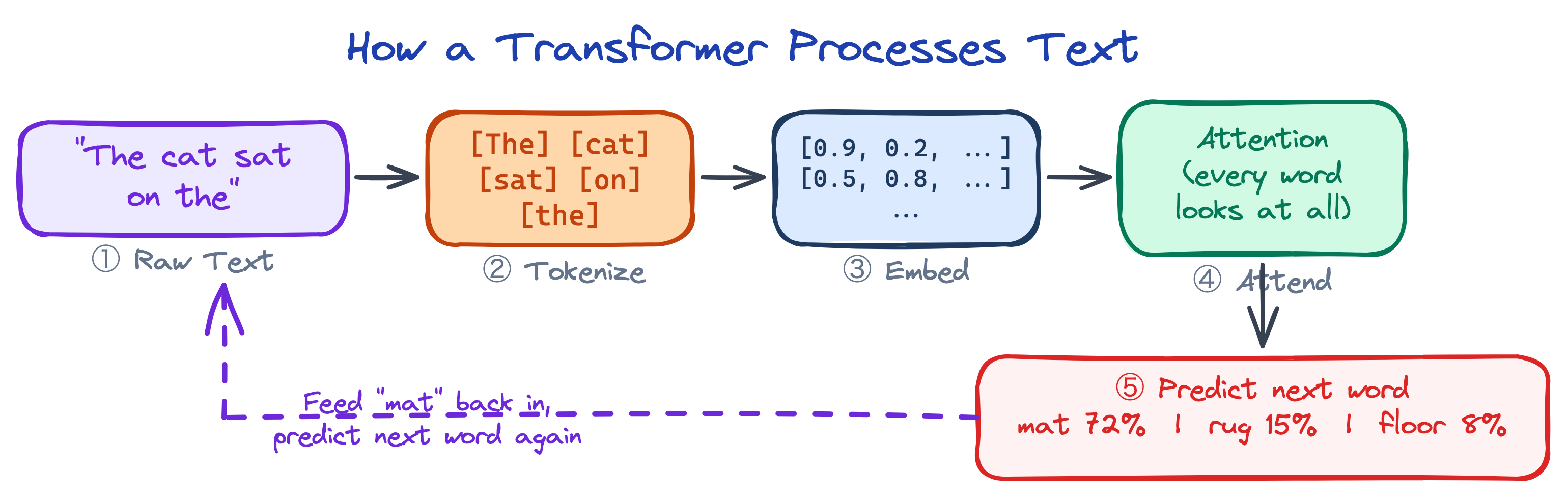
Text in — “The cat sat on the”
Tokenize — break into pieces: [The] [cat] [sat] [on] [the]
Embed — each token becomes a vector of numbers (its meaning)
Attend — every token looks at every other token to understand context
Predict — output a probability for each possible next word

Generating Text: One Word at a Time

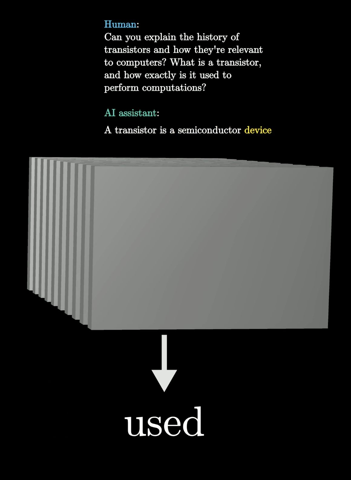
The model takes the full conversation, predicts one word, appends it, and repeats. Every response from ChatGPT, Claude, or Gemini is generated this way — one token at a time, each time looking at everything that came before.

Encoder vs Decoder

The original transformer had two halves:

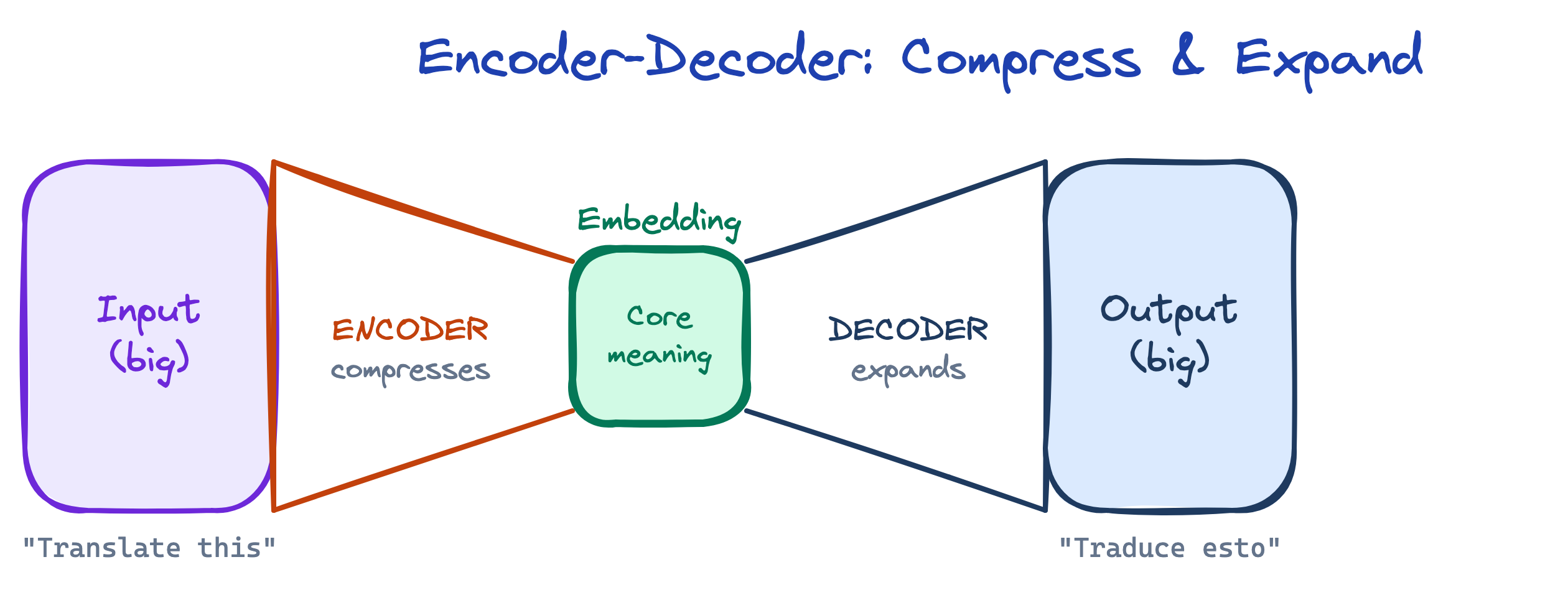
Encoder: reads the input, compresses it into a dense embedding that captures the core meaning
Decoder: takes that embedding and expands it into an output — word by word
The original 2017 paper used both (for translation: English in → embedding → Spanish out)

Why GPT Uses Only the Decoder

Modern LLMs like GPT and Claude dropped the encoder. Why?

The model’s knowledge is already baked into the weights from pretraining on trillions of tokens. It doesn’t need to re-encode your input from scratch — it already understands language.
If you retrained all weights on every new input: (a) it would be impossibly slow — updating trillions of parameters per token, and (b) it would be chaos — each new sentence would overwrite what the model learned from the previous one.
Instead, the weights are frozen after training. The decoder just generates the next token using what it already knows + your prompt as context.

Note

This is why “prompting” matters so much — you’re not teaching the model anything new. You’re steering a frozen model by giving it the right context to generate from.

From Transformers to LLMs

The Scaling Hypothesis

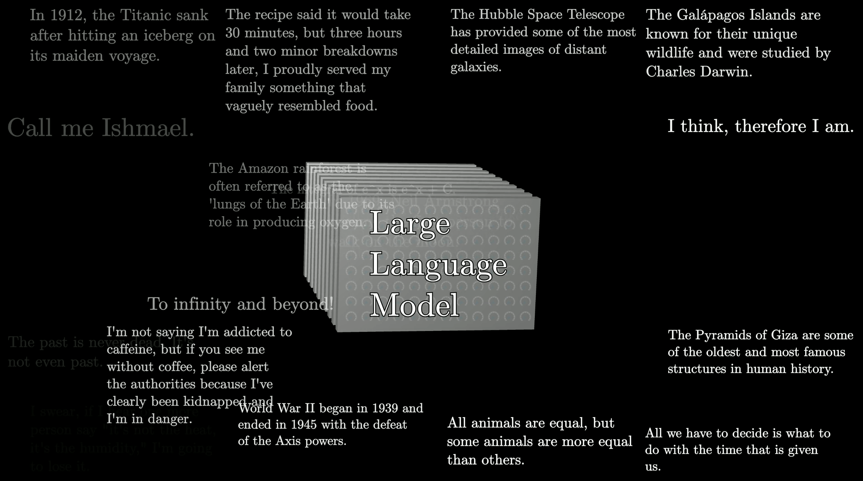
A remarkable discovery: as you increase three things together, performance improves predictably:

More parameters (bigger model)
More data (more text to train on)
More compute (more GPUs, longer training)

Important

Scaling laws mean you can predict how good a model will be before you finish training it. This turned AI from alchemy (“try things and hope”) into engineering (“invest X compute, get Y performance”).

Transfer Learning — Don’t Start From Scratch

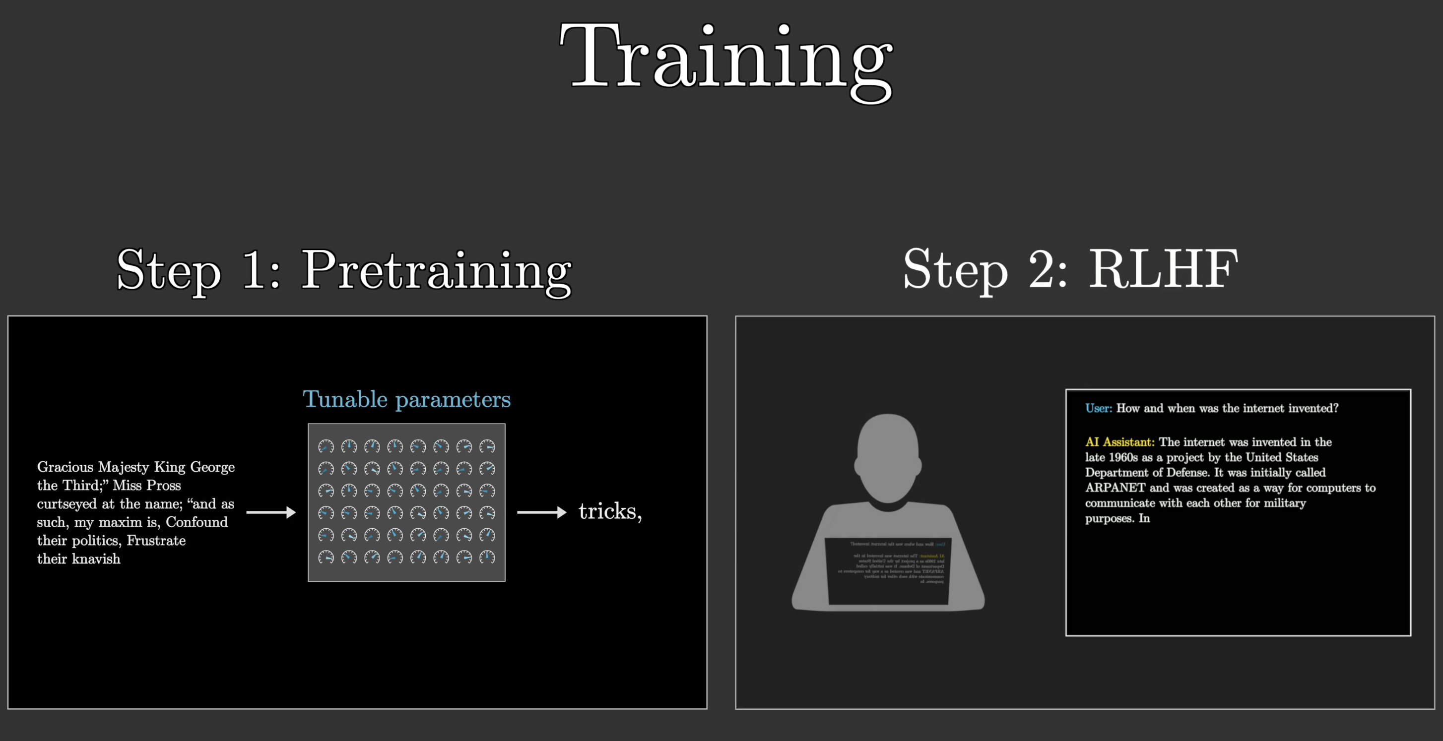
Training a model from zero takes millions of dollars. Instead, take a pretrained model and fine-tune it on your specific task.

GPT was trained on the entire internet → fine-tune it on your company’s support tickets
A vision model trained on millions of images → fine-tune it on your X-ray dataset
This is called transfer learning — reuse what the model already knows

Important

Transfer learning is how most companies actually use AI today. You don’t train a model — you adapt one. This is why foundation models (GPT, Claude, LLaMA) are so valuable: they’re the starting point everyone builds on.

GPT — Predict the Next Word, at Scale

GPT (Generative Pre-trained Transformer) has one training objective: predict the next token.

Given “The cat sat on the,” predict “mat.” That’s it — billions of times, on billions of documents.

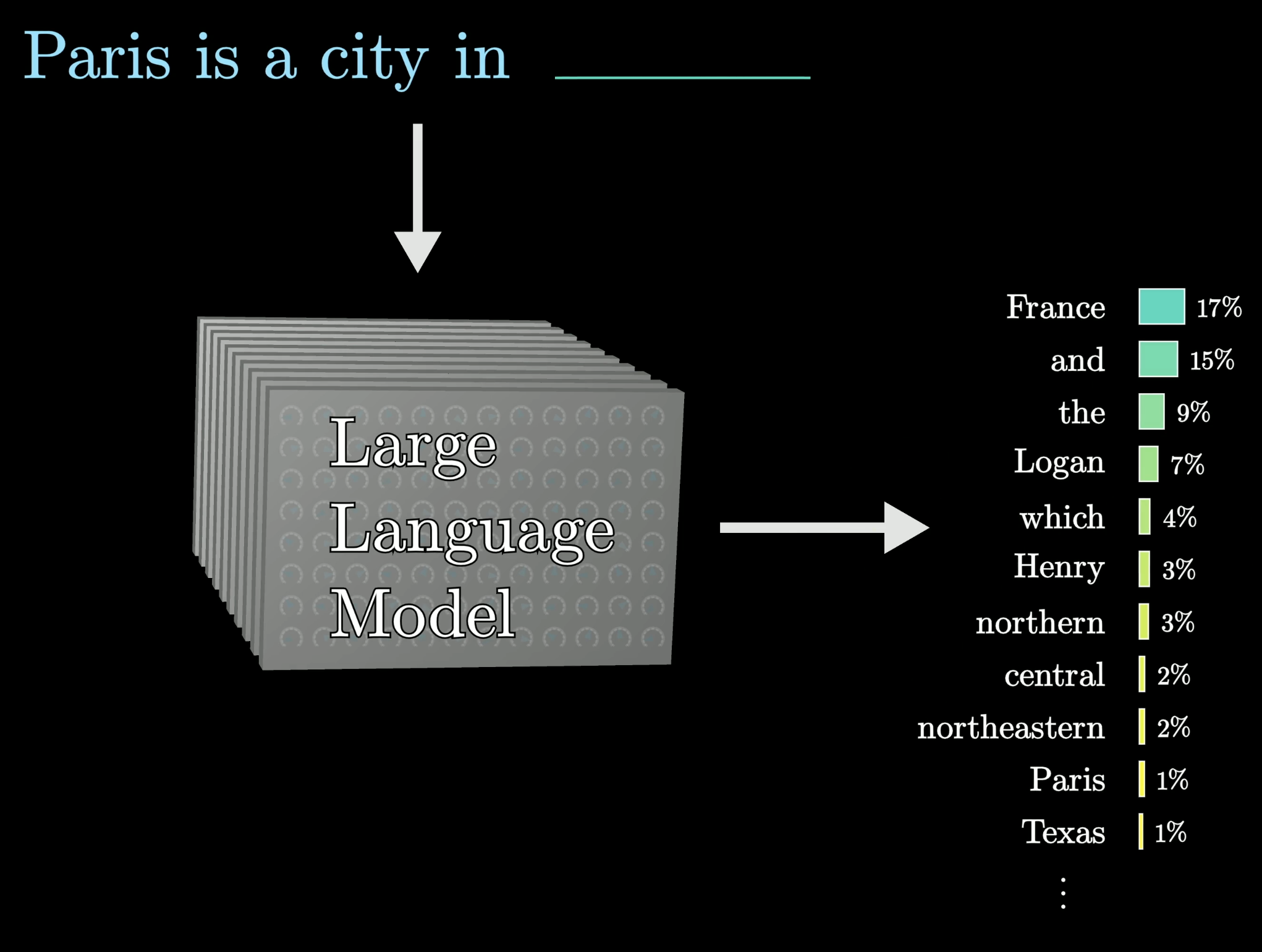
From this simple objective, the model learns grammar, facts, reasoning, and coding — all as a side effect of getting better at prediction.

Note

GPT-1 (2018) had 117 million parameters. GPT-5 (2025) has an estimated 5 trillion. Same idea, 40,000x bigger — and the results went from “interesting toy” to “writes better than most humans.”

Not Just Words — Real Knowledge

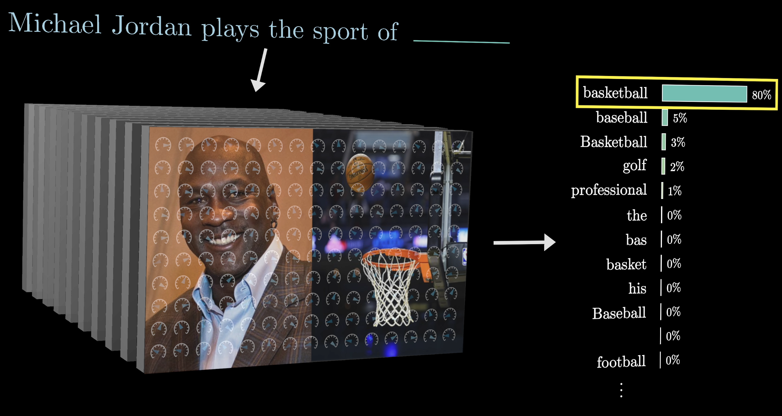
“Michael Jordan plays the sport of ___” → basketball (80%).

This isn’t just word patterns — at scale, the model learns real facts about the world. It knows Michael Jordan plays basketball, that Paris is in France, that water boils at 100°C. All from predicting the next word, billions of times.

Emergent Capabilities

Something unexpected happens as models scale: they develop abilities never explicitly trained on.

Few-shot learning — give it a few examples in the prompt and it infers the task. GPT-3 went from 76% to 86% accuracy on a reading comprehension benchmark just by showing it a handful of examples — no retraining.
- “Scaling up language models greatly improves task-agnostic, few-shot performance” — Brown et al., NeurIPS 2020
Chain-of-thought reasoning — say “think step by step” and it solves multi-step problems. On a math benchmark (GSM8K), accuracy jumped from 18% to 58% — just by changing the prompt. This only works above ~100B parameters. Smaller models show no benefit.
- “Chain-of-thought prompting elicits reasoning in large language models” — Wei et al., 2022
Code generation — GPT-4 was asked to draw a unicorn in TikZ (LaTeX). It had never seen “draw a unicorn in code” — but it combined knowledge of geometry, LaTeX syntax, and what unicorns look like into working code. Researchers could even ask it to fix the horn placement.
- “GPT-4 can solve novel tasks that span mathematics, coding, vision, medicine, law” — Bubeck et al., Microsoft Research, 2023
Translation between unseen pairs — a model trained on English↔︎Portuguese and English↔︎Russian could translate Portuguese↔︎Russian directly — a pair it never saw — by mapping both languages into a shared embedding space.
- “Decoupled vocabulary learning enables zero-shot translation from unseen languages” — ACL 2024

None of these were in the training objective. The model was only trained to predict the next word.

The Current Landscape

Model	Company	Key Feature
GPT-5	OpenAI	Reasoning, multimodal
Claude	Anthropic	Safety-focused, long context
Gemini	Google	Multimodal, integrated with Search
LLaMA	Meta	Open-source, runs locally
Mistral	Mistral AI	Efficient, open-weight

Note

Richard Sutton’s “The Bitter Lesson” (2019) argues: the history of AI shows that general methods that scale with compute ultimately win over methods that try to encode human knowledge. Transformers + scale are the latest proof.

Try It: Next-Word Probabilities

Step 1 of how a language model works — given previous words, what are the probabilities for the next word?

Try It: Attention Scores

Step 2 — attention. Each word builds an embedding from the corpus. To predict the next word, we compute how much each context word “attends to” every other word.

Note

Real transformers do exactly this — but with learned embeddings (not co-occurrence), 96 attention heads running in parallel, and billions of parameters. The mechanism is the same: query the context, score relevance, focus on what matters.

Your Assignment

Train an AI to Play Pac-Man

Important

Build a Deep Q-Learning agent that learns to play Pac-Man — with automatic hardware detection, live gameplay demonstrations, and GIF recordings that show your agent evolving from random chaos to deliberate play.

Implement a Deep Q-Network (DQN) with a convolutional neural network
Auto-detect your hardware — Apple Silicon (MPS), NVIDIA GPU (CUDA), or CPU
Train on the MsPacman Gymnasium/Atari environment
Every 25 episodes, pop open a live game window and save a GIF of the gameplay
Plot training metrics: score over time, loss curve, epsilon decay
No cloud needed — runs entirely on your laptop

This assignment ties together everything from today: neural networks, loss functions, gradient descent, overfitting, and reinforcement learning — except now you’ll see it happening live as Pac-Man gets smarter.

This Is What Episode 0 Looks Like

The untrained agent plays completely randomly — no strategy, no learning, pure chaos:

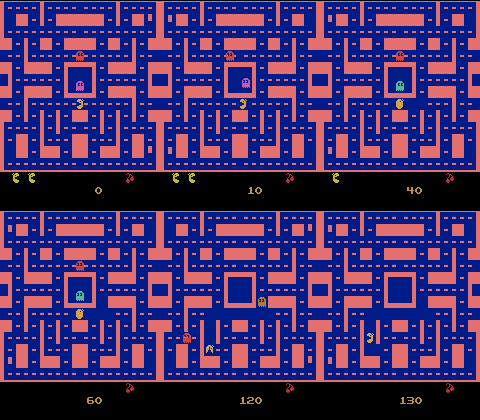
By episode 300+, the same agent will be deliberately eating pellets and avoiding ghosts. Your job: make that happen.

Setup

mkdir pacman-dqn
cd pacman-dqn

# Pick one:
claude --dangerously-skip-permissions   # Claude Code
codex --yolo                            # OpenAI Codex

Note

Requires Python 3.10+. The Atari ROM will be auto-downloaded by Gymnasium’s ALE integration — no manual ROM setup needed.

Installing PyTorch for your platform

macOS (Apple Silicon): pip install torch — MPS support is built-in since PyTorch 2.0
Linux (NVIDIA GPU): pip install torch --index-url https://download.pytorch.org/whl/cu121
Windows / CPU: pip install torch

The project will auto-detect and use the best available device.

The Prompt

Paste this into Claude Code (click Copy then paste):

/plan Build a Deep Q-Learning agent that learns to play Pac-Man.
Use Python only — no web stack. This runs locally on the student's
laptop.

Stack:
- gymnasium[atari,accept-rom-license] for the ALE/MsPacman-v5
  environment
- ale-py (auto-installed with gymnasium[atari])
- AutoROM[accept-rom-license] for Atari ROM files
- PyTorch for the DQN (detect and use best available device)
- matplotlib for training plots
- opencv-python for frame preprocessing
- imageio for saving gameplay GIFs

The project should have these files:

1. device.py — Device detection module:
   - Detect OS via platform.system() (macOS, Linux, Windows)
   - Detect best torch device: CUDA (NVIDIA GPU) → MPS (Apple
     Silicon) → CPU
   - Print a startup banner: OS, device type, torch version
   - Export a DEVICE variable used by all other modules
   - If GPU available, use larger batch size (64 vs 32)

2. model.py — The DQN: a convolutional neural network that takes
   a stack of 4 preprocessed grayscale 84×84 game frames and
   outputs Q-values for each action. Architecture:
   - Conv2d(4, 32, 8, stride=4) → ReLU
   - Conv2d(32, 64, 4, stride=2) → ReLU
   - Conv2d(64, 64, 3, stride=1) → ReLU
   - Flatten → Linear(3136, 512) → ReLU → Linear(512, n_actions)
   - Model lives on the detected device from device.py

3. replay_buffer.py — Experience replay buffer (capacity 100,000)
   that stores (state, action, reward, next_state, done) tuples
   and samples random minibatches.

4. agent.py — The DQN agent with:
   - Epsilon-greedy: start ε=1.0, decay to 0.1 over 100k steps
   - Target network updated every 10,000 steps
   - γ=0.99, lr=1e-4, Adam optimizer, Huber loss
   - All tensors on the device from device.py

5. preprocess.py — Frame preprocessing:
   - Grayscale, resize 84×84, stack 4 frames, normalize to [0,1]

6. train.py — Main training loop:
   - Print device banner at startup (from device.py)
   - BEFORE any training: run a demo of the UNTRAINED agent
     (episode 0) so the student sees pure random play first
   - Train for 500 episodes (or Ctrl+C to stop gracefully)
   - Every 25 episodes: run a VISUAL DEMO episode — render
     frames with render_mode="rgb_array" and display them
     live in a matplotlib window (NOT render_mode="human",
     which doesn't reliably open on macOS). Also save the
     frames as a GIF in demos/ folder
     (demos/episode_0000.gif, demos/episode_0025.gif, etc.)
   - After the demo, print: episode, score, running avg, epsilon
   - Track: episode reward, running avg (last 25), epsilon, loss
   - Save model checkpoint every 100 episodes to checkpoints/
   - On Ctrl+C: save model, generate final plot, print summary

7. play.py — Load a saved model and watch it play:
   - Use matplotlib window to render each game live
     (render_mode="rgb_array" + imshow, NOT "human")
   - Play 5 games, save a GIF of the best to demos/final_best.gif
   - Print scores for each game

8. plot.py — Training dashboard (saved as training_dashboard.png):
   - Episode reward over time + 25-episode moving average
   - Training loss over time
   - Epsilon decay curve

Include requirements.txt with all dependencies.
Include README.md with:
- Platform-specific install instructions (macOS/Linux/Windows + GPU)
- How to train: python train.py
- How to watch: python play.py
- How to plot: python plot.py
- What to expect at each stage
- Estimated training times by device

IMPORTANT: Device detection is critical — the agent should
automatically use the best available hardware. The GIF demos
in demos/ folder are the key deliverable — students should see
their agent evolve from random movement to intentional play.

What to Expect

Training times by device

Device	Estimated time
NVIDIA GPU (CUDA)	~15–25 minutes
Apple Silicon (MPS)	~20–40 minutes
CPU only	~45–90 minutes

Every 25 episodes, a game window pops up and a GIF is saved to demos/:

Episodes 1–50: Random chaos. Pac-Man walks into ghosts.
Episodes 50–150: Starts eating nearby pellets. Still dies a lot.
Episodes 150–300: Learns to avoid ghosts, chases pellets deliberately.
Episodes 300–500: Clears significant portions of the board.

Note

Why this matters: You’re watching everything from today’s class come alive — the neural network learns by minimizing a loss function (Huber loss), uses gradient descent (Adam optimizer), fights overfitting with experience replay, and balances exploration vs exploitation (epsilon-greedy). The GIF timeline in demos/ is your loss curve made visible: a bad agent is high loss.

Submit Your Assignment

→ Submit your homework — sign in with GitHub, submit your GitHub repo URL. Include a screenshot of your training plot and your best gameplay GIF.

Thank You & What’s Next

Thank you for being here — giving up your personal time to learn this. It matters, and it will pay off.

In Class 3, we’ll stop studying how LLMs work and start using them.

→ Class 2 Survey

Help me improve — 1 minute, anonymous.

Next: Class 3 — LLMs in Practice →